Summary: I learn best with toy code that I can play with. This tutorial teaches DeepMind's Neural Stack machine via a very simple toy example, a short python implementation. I will also explain my thought process along the way for reading and implementing research papers from scratch, which I hope you will find useful.
I typically tweet out new blogposts when they're complete at @iamtrask. Feel free to follow if you'd be interested in reading more in the future and thanks for all the feedback!
Part 1: What is a Neural Stack?
A Simple Stack
Let's start with the definition of a regular stack before we get to a neural one. In computer science, a stack is a type of data structure. Before I explain it, let me just show it to you. In the code below, we "stack" a bunch of harry potter books on an (ascii art) table.
Just like in the example above, picture yourself stacking Harry Potter books onto a table. A stack is pretty much the same as a list with one exception: you can't add/remove a book to/from anywhere except the top. So, you can add another to the top ( stack.push(book) ) or you can remove a book from the top ( stack.pop() ), however you can't do anything with the books in the middle. Pushing when we add a book to the top. Popping is when we remove a book from the top (and perhaps do something with it :) )
A Neural Stack
A close eye might ask, "We learn things with neural networks. What is there to learn with a data structure? Why would you learn how to do what you can easily code?" A neural stack is still just a stack. However, our neural network will learn how to use the stack to implement an algorithm. It will learn when to push and pop to correctly model output data given input data.
How will a neural network learn when to push and pop?
A neural network will learn to push and pop using backpropgation. Certainly a pre-requisite to this blogpost is an intuitive understanding of neural networks and backpropagation in general. Everything in this blogpost will be enough.
So, how will a neural network learn when to push and pop? To answer this question, we need to understand what a "correct sequence" of pushing and popping would look like? And that's right... it's a "sequence" of pushing and popping. So, that means that our input data and our correct output data will both be sequences. So, what kinds of sequences are stacks good at modeling?
When we push a sequence onto a stack, and then pop that sequence off of the stack. The squence pops off in reverse order to the original sequence that was pushed. So, if you have a sequence of 6 numbers, pushing 6 times and then popping 6 times is the correct sequence of pushing and popping to reverse a list.
...so What is a Neural Stack?
A Neural Stack is a stack that can learn to correctly accept a sequence of inputs, remember them, and then transform them according to a pattern learned from data.
...and How Does It Learn?
A Neural Stack learns by:
1) accepting input data, pushing and popping it according to when a neural network says to push and pop. This generates a sequence of output data (predictions).
2) Comparing the output data to the input data to see how much the neural stack "missed".
3) Updating the neural network to more correctly push and pop next time. (using backpropagation)
... so basically... just like every other neural network learns...
And now for the money question...
Money Question: How does backpropagation learn to push and pop when the error is on the output of the stack and the neural network is on the input to the stack? Normally we backpropagate the error from the output of the network to the weights so that we can make a weight update. It seems like the stack is "blocking" the output from the decision making neural network (which controls the pushing and popping).
Money Answer: We make the neural stack "differentiable". If you haven't had calculus, the simplest way to think about it is that we will make the "neural stack" using a sequence of vector additions, subtractions, and multiplications. If we can figure out how to mimic the stack's behaviors using only these tools, then we will be able to backpropagate the error through the stack just like we backpropagate it through a neural network's hidden layers. And it will be quite familiar to us! We're already used to backpropagating through sequences of additions, subtractions, and multiplications. Figuring out how to mimic the operations of a stack in a fully differentiable way was the hard part... which why Edward Grefenstette, Karl Moritz Hermann, Mustafa Suleyman, and Phil Blunsom are so brilliant!!!
Part 2: Reading and Implementing Academic Papers
Where To Start....
As promised, I want to give a bit of "meta-learning" regarding how to approach implementing academic papers. So, pop open this paper and have a look around. As a disclaimer, there is no correct way to read academic papers. I wish only to share how I approached this one and why. Feel free to take any/all of it with a grain of salt. If you have lessons to add from experience, please comment on the hacker news or reddit posts if you came from there... or feel free to tweet @iamtrask. I'm happy to retweet good advice on this topic.
First Pass: Most people I know start by just reading a paper start to finish. Don't try to understand everything. Just get the high level goal of what's being accomplished, the key vocabulary terms involved, and a sense of the approach. Don't worry too much about formulas. Take time to look at pictures and tables. This paper has lots of good ones, which is helpful too. :) If this paper were about how to build a car, this first pass is just about learning "We're going to build a driving machine. It's going to be able to move and turn at 60 miles per hour down a curvy road. It runs on gasolean and has wheels. I think it will be driven by a human being." Don't worry about the alternator, transmission, or spark plugs... and certainly not the optimal temperature for combustion. Just get the general idea.
Second Pass: For the second pass, if you feel like you understand the background (which is always the first few sections... commonly labeled "Introduction" and "Related Work"), jump straight to the approach. In this paper the approach section starts with "3 Models" at the bottom of page 2. For this section, read each sentence slowly. These sections are almost always extremely dense. Each sentence is crafted with care, and without an understanding of each sentence in turn, the next might not make sense. At this point, still don't worry too much about the details of the formulas. Instead, just get an idea of the "major moving parts" in the algorithm. Focus on the what not the how. Again, if this were about building a car, this is about making a list of what each part is called and what it generally does like below...
| Part Name | Variable | Description When First Reading |
|---|---|---|
| "The Memory" | V_t | Sortof like "self.contents" in our VerySimpleStack. This is where our stuff goes. More specifically, this is the state of our stack at timestep "t". |
| "The Controller" | ? | The neural network that decides when to push or pop. |
| "Pop Signal" | u_t | How much the controller wants to pop. |
| "Push Signal" | d_t | How much the controller wants to push. |
| "Strength Signal" | s_t | Given u_t and d_t are real valued, it seems like we can push on or pop off "parts" of objects... This vector seems to keep up with how much of each variable we still have in V (or V_t really). |
| "Read Value" | v_t | This seems to be made by combining s_t and V_t somehow.... so some sort of weighted average of what's on the stack... interesting.... |
| "Time" | _t | This is attached to many of the variables... i think it means the state of that variable at a specific timestep in the sequence. |
As a sidenote, this is also a great time to create some mental pneumonics to remember which variable is which. In this case, since the "u" in "u_t" is open at the top... I thought that it looked like it has been "popped" open. It's also the "pop signal". In contrast, "d_t" is closed on top and is the "push signal". I found that this helped later when trying to read the formulas intuitively (which is the next step). If you don't know the variables by heart, it's really hard to figure out how they relate to each other in the formulas.
N More Passes: At this point, you just keep reading the method section until you have your working implementation (which you can evaluate using the later sections). So, this is generally how to read the paper. :)
Have Questions? Stuck? Feel free to tweet your question @iamtrask for help.
Part 3: Building a Toy Neural Stack
Where To Start....
Ok, so we have a general idea of what's going on. Where do we start? I'm always tempted to just start coding the whole big thing but inevitably I get halfway through with bugs I'll never find again. So, a word from experience, break down each project into distinct, testable sections. In this case, the smallest testable section is the "stack mechanism" itself. Why? Well, the bottom of page 5 gives it away "the three memory modules... contain no tunable parameters to optimize during training". In a word, they're deterministic. To me, this is always the easiest place to start. Debugging something with deterministic, constant behavior is always easier than debugging something you learn/optimize/constantly changes. Furthermore, the stack logic is at the core of the algorithm. Even better, Figure 1 section (a) gives its expected behavior which we can use as a sort of "unit test". All of these things make this a great place to start. Let's jump right into understanding this portion by looking at the diagram of the stack's architecture.
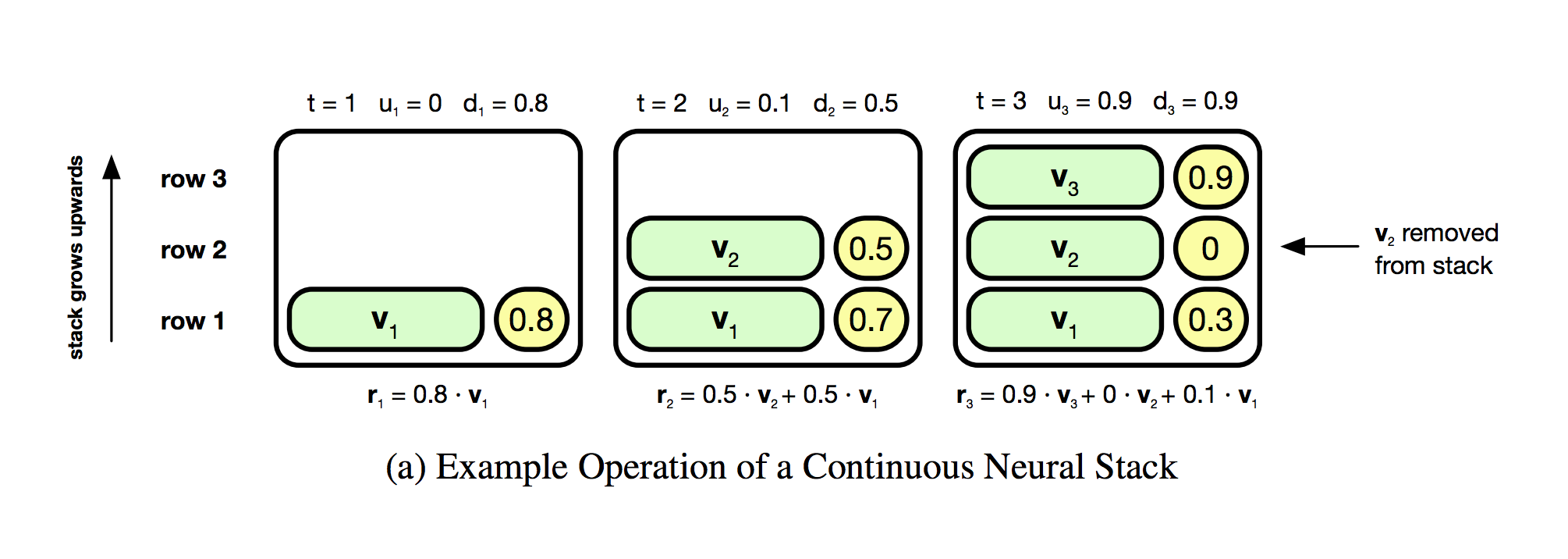
What I'm Thinking When I See This: Ok... so we can push green vectors v_t onto the stack. Each yellow bubble on the right of each green v_t looks like it coresponds to the weight of v_t in the stack... which can be 0 apparently (according to the far right bubble). So, even though there isn't a legend, I suspect that the yellow circles are infact s_t. This is very useful. Furthermore, it looks like the graphs go from left to right. So, this is 3 timesteps. t=1, t=2, and t=3. Great. I think I see what's going on.
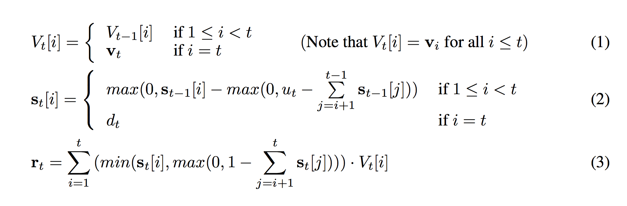
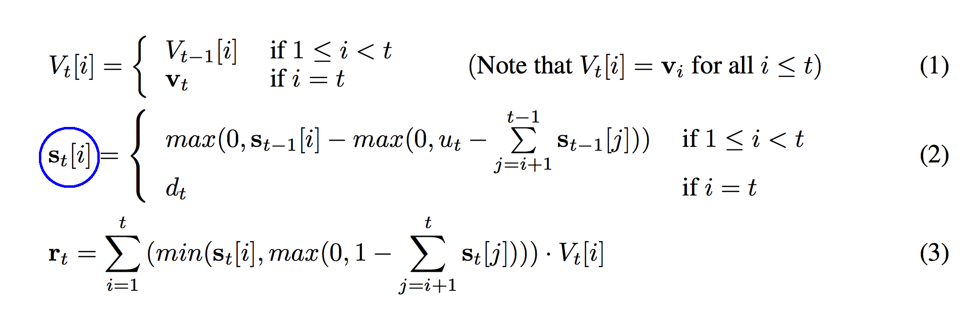
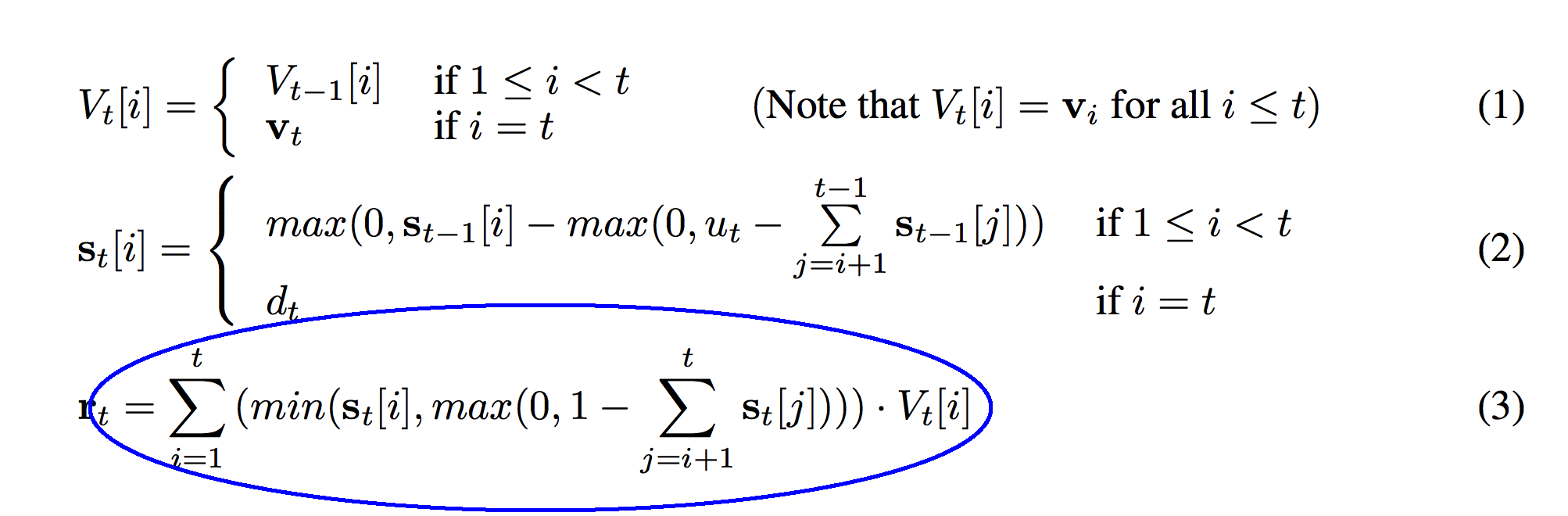
What I'm Thinking: Ok. I can line up the formulas with the picture above. The first formula sets each row of V_t which are the green bubbles. The second formula determines each row of s_t, which are the yellow bubbles. The final formula doesn't seem to be pictured above but I can see what its values are given the state of the stack. (e.g. r_3 = 0.9 * v_3 + 0 * v_2 + 0.1 * v_1) Now, what are these formulas really saying?
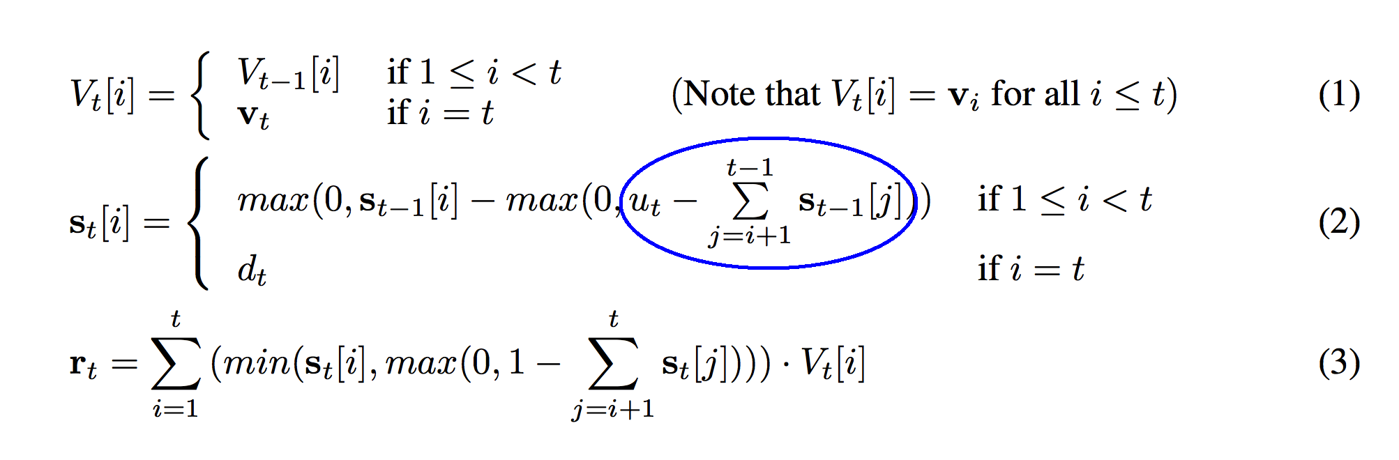
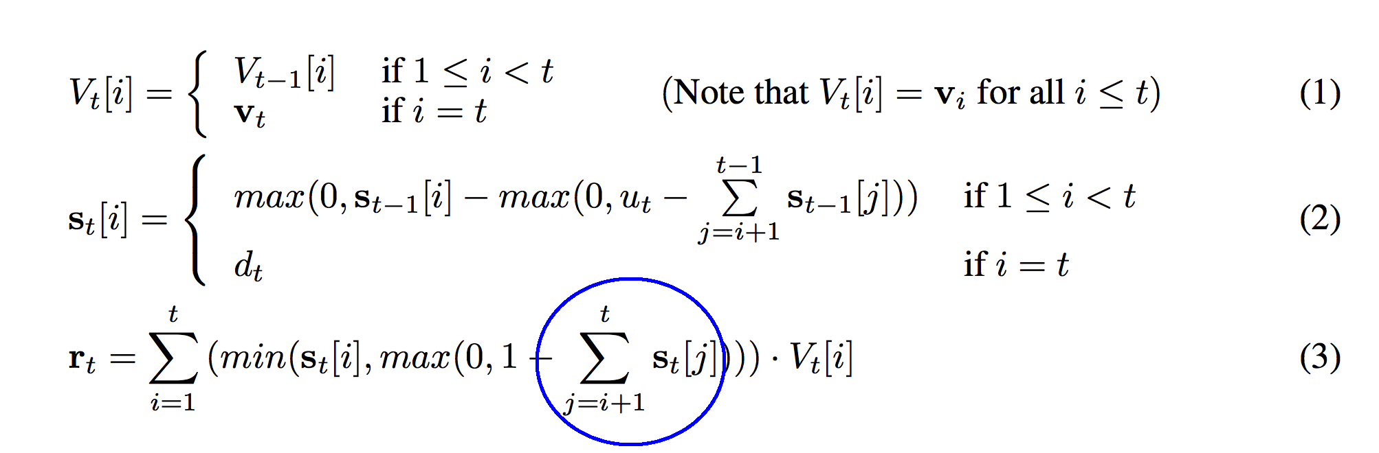
So, what we're going to try to do here is "tell the story" of each part of each formula in our head. Let's start with the first formula (1) which seems the least intimidating.
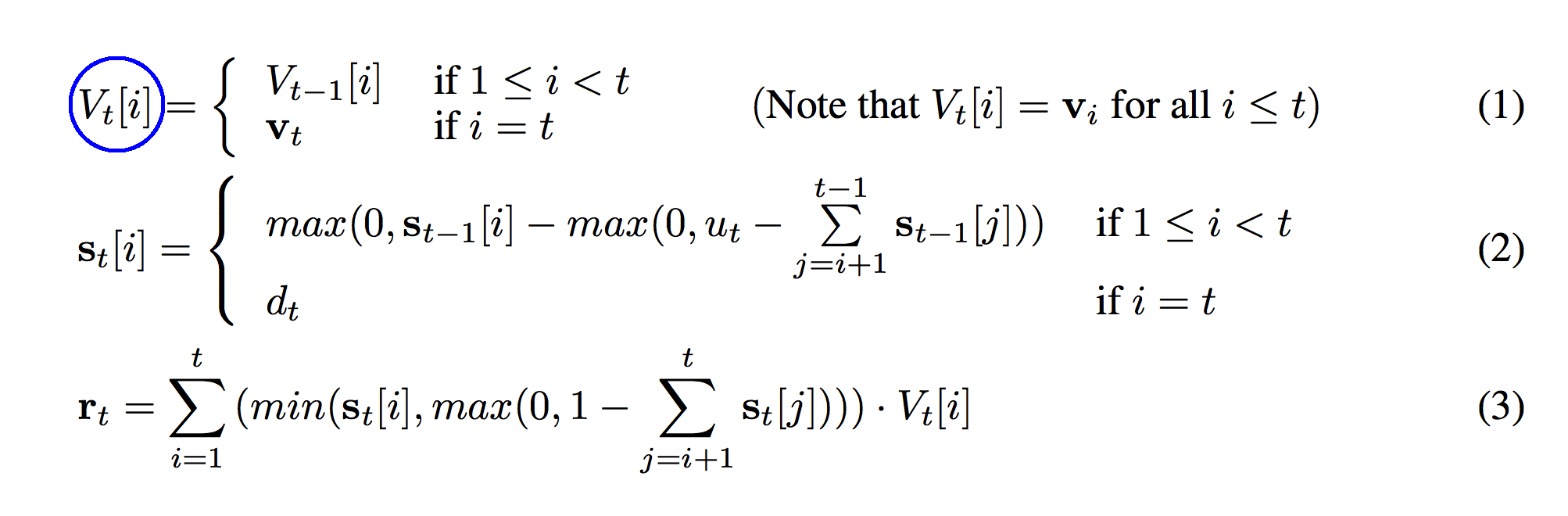
See the part circled in blue above? Notice that it's indexed by two numbers, t, and i. I actually overlooked this at first and it came back to bite me. V_t is the state of our stack's memory at time t. We can see its state in the picture at t=1, t=2, and t=3. However, at each timestep, the memory can have more than one value v_t inside of it! This will have significant implications for the code later (and the memory overhead).
Bottom Line: If V_t is the state of the stack's memory at time "t", then V is a list of ALL of the memory states the stack goes through (at every timestep). So, V is a list of lists of vectors. (a vector is a list of numbers). In your head, you can think of this as the shape of V. Make sure you can look away and tell yourself what the shapes of V, V_t, and V_t[i] are. You'll need that kind of information on the fly when you're reading the rest of the paper.
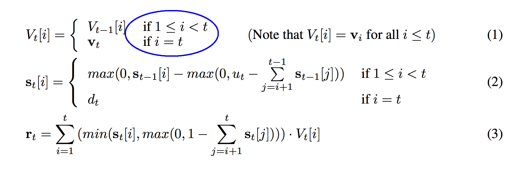
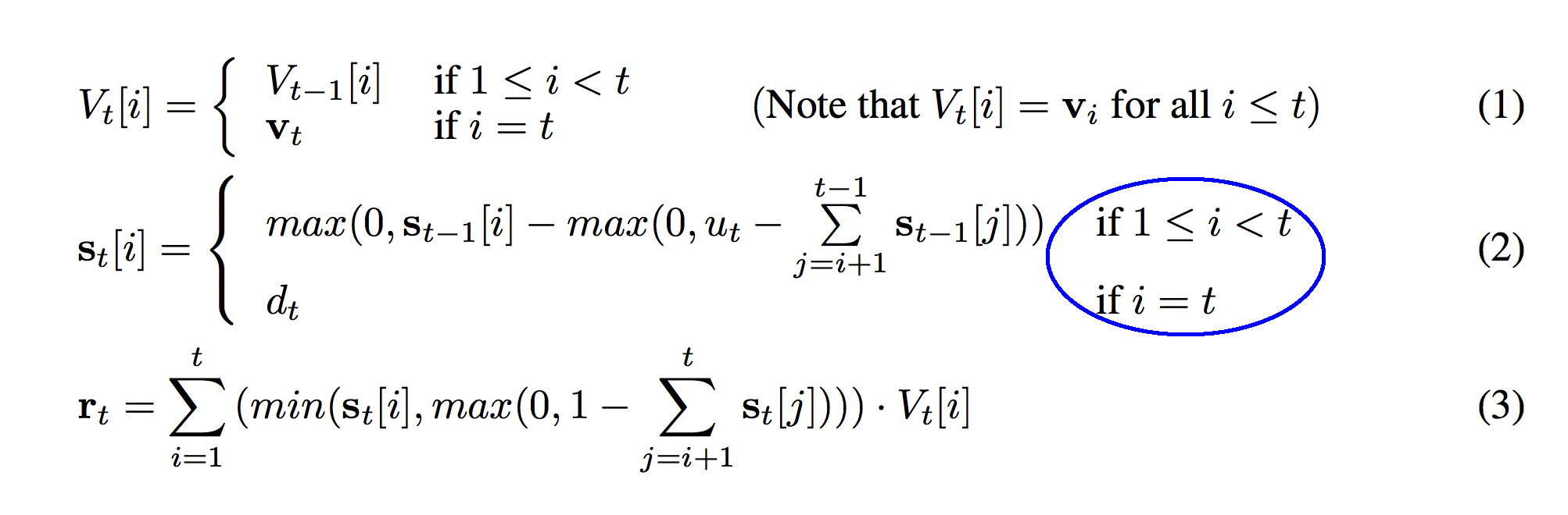
Ok, so this next section defines a conditional function. In this case, that means that the function is different depending on what value "i" takes on. If our variable "i" is greater than or equal to 1 AND is less than t, then V_t[i] = V_t-1[i]. If, on the other hand, "i" equals "t", then V_t[i] = v_t.
So, what story is this telling? What is really going on? Well, what are we combining to make V_t[i]? We're either using V_t-1 or v_t. That's interesting. Also, since "i" determines each row of the stack, and we've got "if" statements depending on "i", that means that different rows of the stack are created differently. If "i" == "t"... which would be the newest member of the stack... then it's equal to some variable v_t. If not, hoever, then it seems like it equals whatever the previous timestep equaled at that row. Eureka!!!
So, all this formula is really saying is... each row of V_t is the same as it was in the previous timestep EXCEPT for the newest row v_t... which we just added! This makes total sense given that we're building a stack! Also, when we look at the picture again, we see that each timestep adds a new row... which is curious.
Interesting... so we ALWAYS add a row. We ALWAYS add v_t. That's very interesting. This sounds like we're always pushing. V_t has t rows. That must be why "i" can range from 1 to "t". We have "t" rows for "i" to index.
Take a deep breath. This formula is actually pretty simple, although there are a few things to note that could trip us up in the implementation. First, "i" doesn't seem to be defined at 0 (by "not defined" i mean that they didn't tell us what to do if i == 0... so what do we do?). To me, this means that the original implementation was probably written in Torch (Lua) instead of Theano (Python) because "i" seems to range from 1 to t (as opposed to 0 to t). "i" is an index into an array. In Lua, the first value in an array or list is at index 1. In Python (the language we're prototyping in), the first value in an array or list is at index 0. Thus, we'll need to compensate for the fact that we're coding this network in a different langauge from the original by subtracting 1 from each index. It's a simple fix but perhaps easy to miss.
So, now that we finished the first formula, can you tell what shape s_t[i] is going to be? It's also indexed by both t and i. However, there's a key difference. The "s" is lowercased which means that s_t is a vector (whereas V_t was a list of vectors... e.g. a matrix). Since s_t is a vector, then s_t[i] is a value from that vector. So, what's the shape of "s"? It's a list of "t" vectors.It's a matrix. (I suppose V is technically a strange kind of tensor.)
def s_t(i,t,u,d):
    if(i >= 0 and i < t):
        inner_sum = sum(s[t-1][i+1:t])
        out = max(0,s[t-1][i] - max(0,u[t] - (inner_sum)))
        return out
    elif(i == t):
        return d[t]
    else:
        print "Undefined i -> t relationship"
When whe just do an exact representation of the function in code, we get the following function above.
This should be very familiar. Just like the first formula (1), formula (2) is also a conditional function based on "i" and "t". They're the same conditions so I suppose there's no additional explanation here. Note that the same 1 vs 0 indexing discrepancy between Lua and Python applies here. In the code, this blue circle is modeled on line 02.
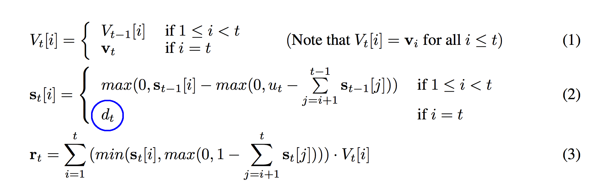
So, we have two conditions that are identical as before. This means that the bottom part of the function (circled in blue) is only true if "i" == "t". "i" only equals "t" when we're talking about the row corresponding to the newest vector on our stack. So, what's the value of s_t for the newest member of our stack? This is where we remember back to the definitions we wrote out earlier. s_t was the strength/weight of each vector on the stack. d_t was our pushing weight. s_t is the current strength. d_t is the weight we pushed it on the stack with.
Pause here... try to figure it out for yourself. What is the relationship between s_t[i] and d_t when i == t?
Aha! This makes sense! For the newest vector that we just put on the stack (V_t[t]), it is added to the stack with the same weight (s_t[i]) that we push it onto the stack with (d_t). That's brilliant! This also answers the question of why we push every time! "not pushing" just means "pushing" with a weight equal to 0! (e.g. d_t == 0) If we push with d_t equal to zero then the weight of that vector on the stack is also equal to 0. This section is represented on line 07 in the code.
def s_t(i,t,u,d):
    if(i >= 0 and i < t):
        inner_sum = sum(s[t-1][i+1:t])
        out = max(0,s[t-1][i] - max(0,u[t] - (inner_sum)))
        return out
    elif(i == t):
        return d[t]
    else:
        print "Undefined i -> t relationship"
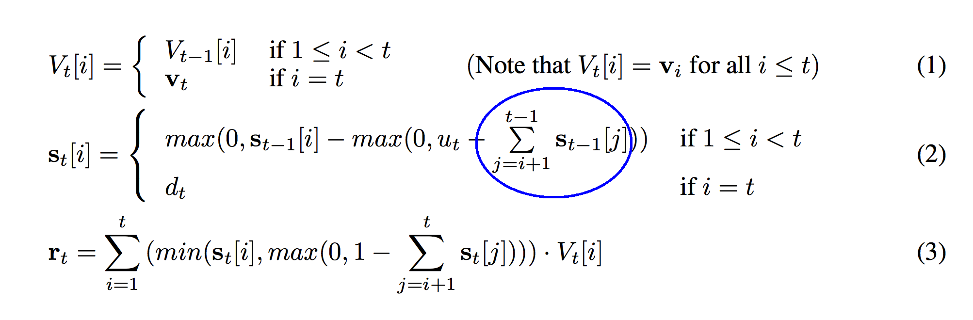
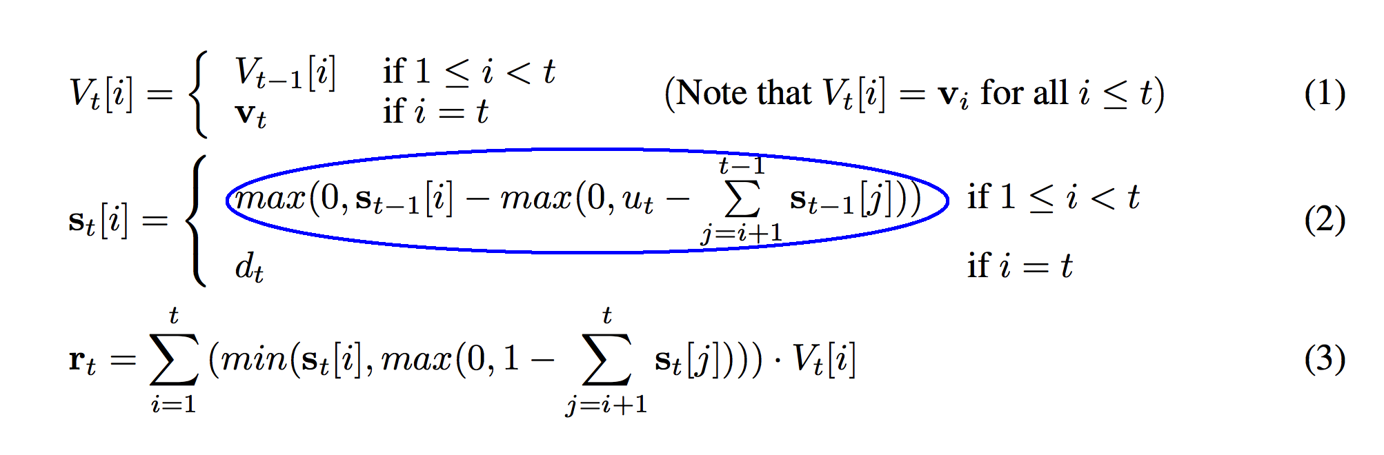
Ok, now we're getting to the meat of a slightly more complicated formula. So, we're gong to break it into slightly smaller parts. I'm also re-printing the picture below to help you visualize the formula. This sum circled in blue sums from i+1 to t-1. Intuitively this is equivalent to summing "all of the weights between s_t[i] and the top of the stack". Stop here. Make sure you have that in your head.
Why t-1? Well, s_t-1 only runs to t-1. s_t-1[t] would overflow.
Why i+1? Well, think about being at the bottom of the ocean. Imagine that s_t is measuring the amount of water at each level in the ocean. Imagine then that the sum circled in blue is measuring "the weight of the water above me". I don't want to include the water even with me when measuring the "sum total amount of water between me and the ocean's surface." Perhaps I only want to measure the water that's "between me and the surface". That's why we start from i+1. I know that's kindof a silly analogy, but that's how I think about it in my head.
So, what's circled in blue is "the sum total amount of weight between the current strength and the top of the stack". We don't know what we're using it for yet, but just remember that for now.
def s_t(i,t,u,d):
    if(i >= 0 and i < t):
        inner_sum = sum(s[t-1][i+1:t])
        out = max(0,s[t-1][i] - max(0,u[t] - (inner_sum)))
        return out
    elif(i == t):
        return d[t]
    else:
        print "Undefined i -> t relationship"
In the code, this blue circle is represented on line 03. It's stored in the variable "inner_sum".
Look below at the circle in the next image. This is only a slight modification to the previous circle. So, if the previous circle was "the sum total amount of weight between the current strength adn the top of the stack", this is "u_t" minus that weight. Remember what u_t was? It's our pop weight! So, this circle is "the amount we want to pop MINUS the weight between the current index and the top of the stack". Stop here and make sure you can picture it.
What does the blue circle above mean intuitively? Let's try the ocean floor analogy again except this time the ocean is dirt. You're buried alive. The sum from before is the sum total amount of weight above you. It's the sum total of all the dirt above you. u_t is the amount of dirt that can be "popped" off. So, if you're popping more than the amount of dirt above you, then this blue circle returns a positive number. You'll be uncovered! You'll be free! However, if u_t is smaller than the amount of dirt above you, then you'll still be buried. The circle will return "-1 * amount_of_dirt_still_above_me". This circle determines how deep in the dirt you are after dirt was popped off. Negative numbers mean you're still buried. Positive numbers mean you're above the ground. The next circle will reveal more about this. Stop and make sure you've got this in your head.
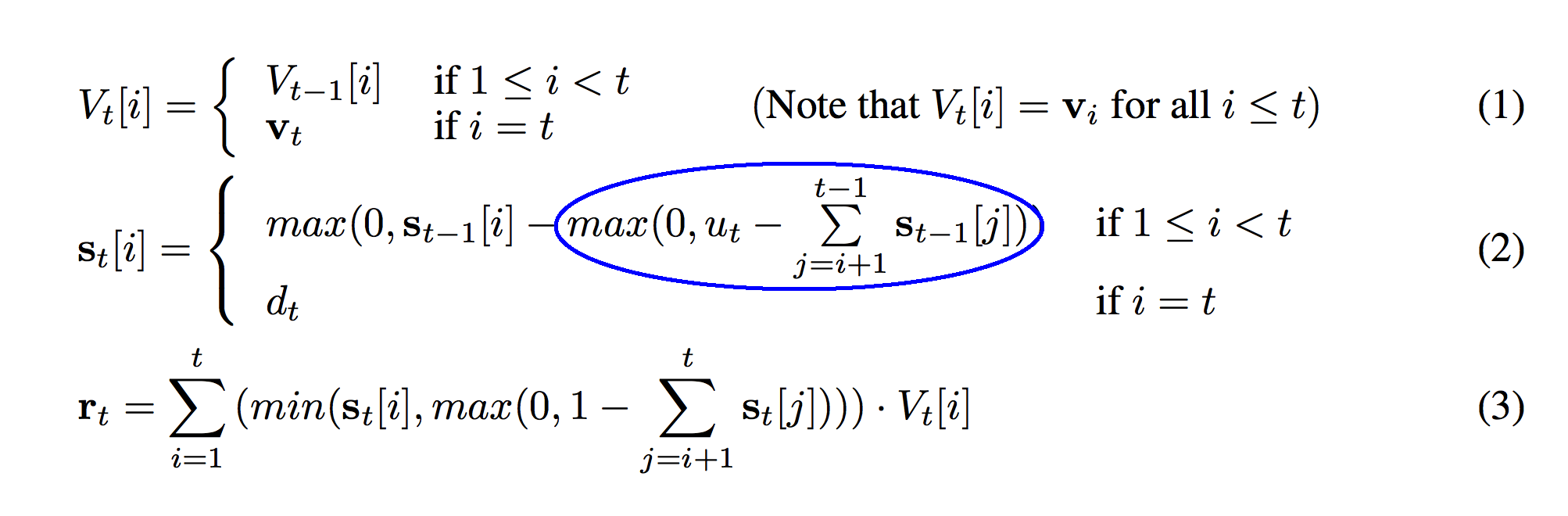
Now instead of picturing yourself as being under the ground, picture yourself as a gold digger from above ground. You're wanting to figure out how far you have to dig to get to some gold. You ask yourself, "if I did 10 meters, how much (if any) gold will I get). u_t is the 10 meters you're digging. The sum previously discussed is the distance from the gold to the surface of the ground. In this case, if u_t - the sum is negative, then you get no gold. If it is positive, then you get gold. That's why we take the max. At each level, we want to know if that vector will be popped off at all. Will the gold at that level be "removed" by popping "u_t" distance. Thus, this circle takes the "max between the difference and 0" so that the output is either "how much gold we get" or "0". The output is either "we're popping off this much" or it's "0". So, the "max" represents how much we have left to "pop" at the current depth in the stack. Stop here and make sure you've got this in your head.
def s_t(i,t,u,d):
    if(i >= 0 and i < t):
        inner_sum = sum(s[t-1][i+1:t])
        out = max(0,s[t-1][i] - max(0,u[t] - (inner_sum)))
        return out
    elif(i == t):
        return d[t]
    else:
        print "Undefined i -> t relationship"
Can you see the second "max" function on line 04. It is the code equivalent of the circled function above
.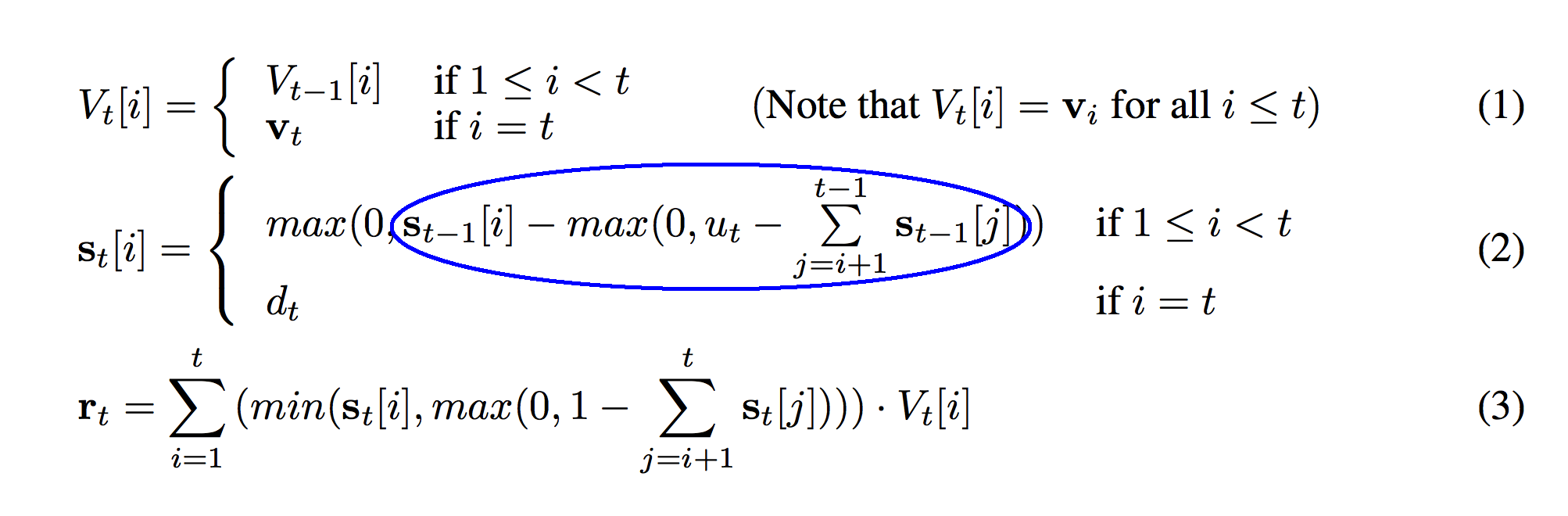
Almost there! So, if the max from the previous circle indicates "whether u_t is large enough to pop this row off (and if so how much of it)", then s_t-1[i] - that number is how much we have left after popping.
If the previous circle was "how much left we have after popping", then this just guarantees that we can only have a positive amount left, which is exactly the desirable property. So, this function is really saying: given how much we're popping off at this time step (u_t), and how much is between this row and the top of the stack, how much weight is left in this row? Note that u_t doesn't have any affect if i == t. (It has no affect on how much we push on d_t) This means that we're popping before we push at each timestep. Stop here and make sure this makes sense in your head.
And now onto the third formula! This sum should look very familiar. The only difference between this sum and the sum in function (2) is that in this function we sum all the way to "t" instead of stopping at "t-1". This means that we're including the most recently pushed strength (s_t) in the sum. Previously we did not.
def r_t(t):
    r_t_out = np.zeros(stack_width)
    for i in xrange(0,t+1):
        temp = min(s[t][i],max(0,1 - sum(s[t][i+1:t+1])))
        r_t_out += temp * V[t][i]
    return r_t_out
The circled sum above is represented with the "sum" function on line 04 of this code. The circled (1 - sum) immediately below this paragraph is equivalent to the (1 - sum) on line 04.
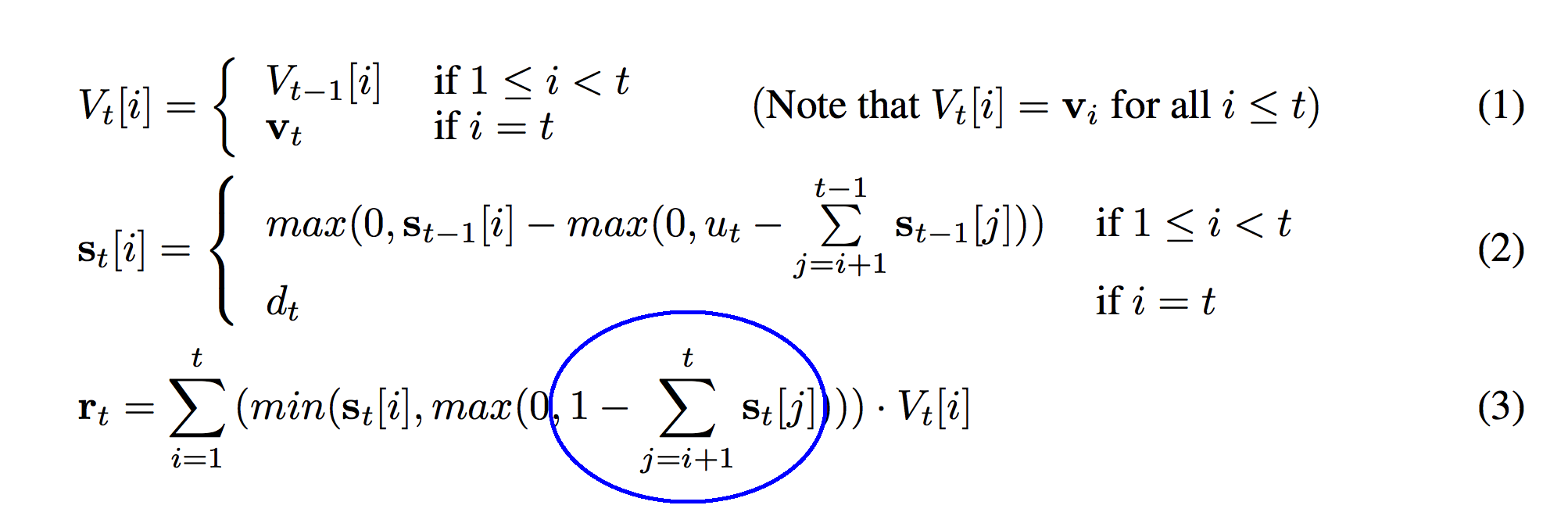
This "1" means a lot more than you might think. As a sneak peek, this formula is reading from the stack. How many vectors is it reading? It's reading "1" deep into the stack. The previous sum calculates (for every row of s_t) the sum of all the weights above it in the stack. The sum calculates the "depth" if you were of each strength at index "i". Thus, 1 minus that strength calculates what's "left over". This difference will be positive for s_t[i] values that are less than 1.0 units deep in the stack. It will be negative for s_t[i] values that are deeper in the stack.
Taking the max of the previous circle guarantees that it's positive. The previous circle was negative for s_t[i] values that were deeper in the stack than 1.0. Since we're only interested in reading values up to 1.0 deep in the stack, all the weights for deeper values in the stack will be 0.
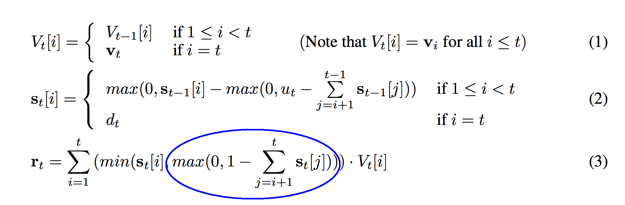
If the previous circle returned 1 - the sum of the weights above a layer in the stack, then it guarantees that the weight is 0 if the layer is too deep. However, if the vector is much shallower than 1.0, the previous circle would return a very positive number (perhaps as high as 1 for the vector at the top). This min function guarantees that the weight at this level doesn't exceed the strength that was pushed onto this level s_t[i].
def r_t(t):
    r_t_out = np.zeros(stack_width)
    for i in xrange(0,t+1):
        temp = min(s[t][i],max(0,1 - sum(s[t][i+1:t+1])))
        r_t_out += temp * V[t][i]
    return r_t_out
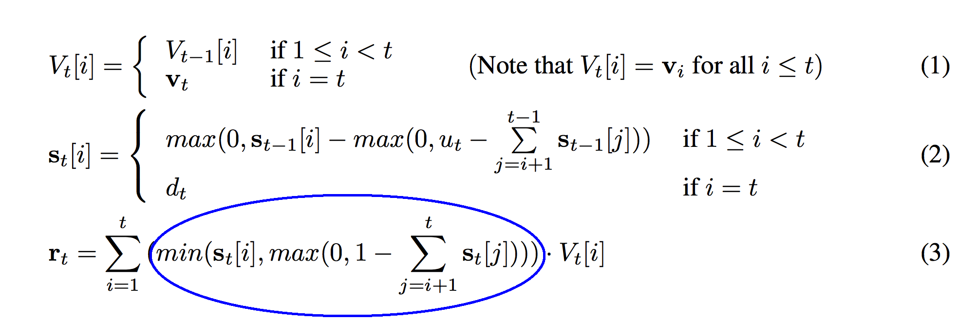
So, the circle in the image above is represented as the variable "temp" created on line 04. The circled section below is the output of the entire function, stored as "r_t_out".
So, what does this function do? It performs a weighted sum over the entire stack, multiplying each vector by s_t, if that vector is less than 1.0 depth into the stack. In other words, it reads the top 1.0 weight off of the stack by performing a weighted sum of the vectors, weighted by s_t. This is the vector that is read at time t and put into the variable r_t.
Writing the Code
Ok, so now we have an intuitive understanding of what these formulas are doing. Where do we start coding? Recall the following figure.
Let's recreate this behavior given the values of u_t, d_t, and r_t above. Remember that many of the "time indices" will be decreased by 1 relative to the Figure 1 above because we're working in Python (instead of Lua).
So, at risk of re-explaining all of the logic above, I'll point to which places in the code correspond to each function.
Lines 1 - 18 initialize all of our variables. v_0, v_1, and v_2 correspond to v_1, v_2, and v_3 in the picture of a stack operating. I made them be the rows of the identity matrix so that they'd be easy to see inside the stack. v_0 has a 1 in the first position (and zeros everywhere else). v_1 has a 1 in the second position, and v_2 has a 1 in the third position.
Lines 13-17 create our basic stack variables... all indexed by "t"
Lines 19-24 correspond to function (3).
Lines 26-33 correspond to function (2).
Lines 35-56 performs a push and pop operation on our stack
Lines 45-55 correspond to function (1). Notice that function (1) is more about how to create V_t given V_t-1.
Lines 58-60 run and print out the exact operations in the picture from the paper. Follow along to make sure you see the data flow!
Lines 62-66 reset the stack variables so we can make sure we got the outputs correct (by making sure they equal the values from the paper)
Lines 68-70 assert that the operations from the graph in the paper produce the correct results
Have Questions? Stuck? Feel free to tweet your question @iamtrask for help.
Part 4: Learning A Sequence
In the last section, we learned the intuitions behind the neural stack mechanism's formulas. We then constructed those exact formulas in python code and validated that they behaved identically to the example laid out in Figure 1 (a) of the paper. In this section, we're going to dig further into how the neural stack works. We will then teach our neural stack to learn a single sequence using backpropagation.
Let's Revisit How The Neural Stack Will Learn
In Part 2, we discussed how the neural stack is unique in that we can backpropgate error from the output of the stack back through to the input. The reason we can do this is that the stack is fully differentiable. (For background on determining whether a function is differentiable, please see Khan Academy . For more on derivatives and differentiability, see the rest of that tutorial.) Why do we care that the stack (as a function) is differentiable? Well, we used the "derivative" of the function to move the error around (more specifically... to backpropagate). For more on this, please see the Tutorial I Wrote on Basic Neural Networks, Gradient Descent, and Recurrent Neural Networks. I particularly recommend the last one because it demontrates backpropgating through somewhat more arbitrary vector operations... kindof like what we're going to do here. :)
Perhaps you might say, "Hey Andrew, pre-requisite information is all nice and good... but I'd like a little bit more intuition on why this stack is differentiable". Let me try to simplify most of it to a few easy to use rules. Backpropagation is really about credit attribution. It's about the neural network saying "ok... I messed up. I was supposed to predict 1.0 but i predicted 0.9. What parts of the function caused me to do this? What parts can I change to better predict 1.0 next time?". Consider this problem.
y = a + b
What if I told you that when we ran this equation, y ended up being a little bit too low. It should have been 1.0 and it was 0.9. So, the error was 0.1. Where did the error come from? Clearly. It came from both a and b equally. So, this gives us an early rule of thumb. When we're summing two variables into another variable. The error is divided evenly between the sum... becuase it's both their faults that it missed! This is a gross oversimplification of calculus, but it helps me remember how to do the chain rule in code on the fly... so I dunno. I find it helpful... at least as a pneumonic. Let's look at another problem.
y = a + 2*b
Same question. Different answer. In this case, the error is 2 times more significant because of b. So remember, when you are multiplying in the function, you have to multiply the error at any point by what that point was multiplied by. So, if the error at y is 0.1. The error at a is 0.1 and the error at b is 2 * 0.1 = 0.2. By the way, this generalizes to vector addition and multiplication as well. Consider in your head why the error would be twice as significant at b. Y is twice as sensitive to changes in b!
y = a*b
Ok, last one for now. If you compute 0.1 error at y, what is the error at a. Well, we can't really know without knowing what b is because b is determining how sensitive y is to a. Funny enough the reverse is also true. a is determining how sensitive y is to b! So, let's take this simple intuition and reflect on our neural stack in both the formal math functions and the code. (Btw, there are many more rules to know in Calculus, and I highly recommend taking a course on it from Coursera or Khan Academy, but these rules should pretty much get you through the Neural Stack)
def s_t(i,t,u,d):
    if(i >= 0 and i < t):
        inner_sum = sum(s[t-1][i+1:t])
        out = max(0,s[t-1][i] - max(0,u[t] - (inner_sum)))
        return out
    elif(i == t):
        return d[t]
    else:
        print "Undefined i -> t relationship"

def r_t(t):
    r_t_out = np.zeros(stack_width)
    for i in xrange(0,t+1):
        temp = min(s[t][i],max(0,1 - sum(s[t][i+1:t+1])))
        r_t_out += temp * V[t][i]
    return r_t_out
Read through each formula. What if the output of our python function r_t(t) was supposed to be 1.0 and it returned 0.9. We would (again) have an error of 0.1. Conceptually, this means we read our stack (by calling the function r_t(t)) and got back a number that was a little bit too low. So, can you see how we can take the simple rules above and move the error (0.1) from the output of the function (line 16) back through to the various inputs? In our case, those inputs include global variables s and V. It's really not any more complicated than the 3 rules we identified above! It's just a long chain of them. This would end up putting error onto s and V. This puts error onto the stack! I find this concept really fascinating. Error in memory! It's like telling the network "dude... you remembered the wrong thing man! Remember something more relevant next time!". Pretty sweet stuff.
So, if we were to code up this error attribution... this backpropagation. It would look like the following.
def s_t_error(i,t,u,d,error):
    if(i >= 0 and i < t):
        if(s_t(i,t,u,d) >= 0):
            s_delta[t-1][i] += error
            if(max(0,u[t] - np.sum(s[t-1][i+1:t-0])) >= 0):
                u_delta[t] -= error
                s_delta[t-1][i+1:t-0] += error
    elif(i == t):
        d_delta[t] += error
    else:
        print "Problem"

def r_t_error(t,r_t_error):
    for i in xrange(0, t+1):
        temp = min(s[t][i],max(0,1 - np.sum(s[t][i+1:t+1])))
        V_delta[t][i] += temp * r_t_error
        temp_error = np.sum(r_t_error * V[t][i])

        if(s[t][i] < max(0,1 - np.sum(s[t][i+1:t+1]))):
            s_delta[t][i] += temp_error
        else:
            if(max(0,1 - np.sum(s[t][i+1:t+1])) > 0):
                s_delta[t][i+1:t+1] -= temp_error # minus equal because of the (1-).. and drop the 1
Notice that I have variables V_delta, u_delta, and s_delta that I put the "errors" into. These are identically shaped variables to V, u, and s respectively. It's just a place to put the delta (since there are already meaningful variables in the regular V, u, and s that I don't want to erase).
From Error Propagation To Learning
Ok, so now we know how to move error around through two of our fun stack functions. How does this translate to learning? What are we trying to learn anyway?
Let's think back to our regular stack again. Remember the toy problem we had before? If we pushed an entire sequence onto a stack and then popped it off, we'd get the sequence back in reverse. What this requires is the correct sequence of pushing and popping. So, what if we pushed 3 items on our stack, could we learn to correctly pop them off by adjusting u_t? Let's give it a shot!
Step one is to setup our problem. We need to pick a sequence, and initialize our u_t and d_t variables. (We're initializing both, but we're only going to try to adjust u_t). Something like this will do.
u_weights = np.array([0,0,0,0,0,0.01])
d_weights = np.array([1,1,1,0,0,0]).astype('float64')
# for i in xrange(1000):
stack_width = 2
copy_length = 5

sequence = np.array([[0.1,0.2,0.3],[0,0,0]]).T

# INIT
V = list() # stack states
s = list() # stack strengths
d = list() # push strengths
u = list() # pop strengths

V_delta = list() # stack states
s_delta = list() # stack strengths
d_delta = list() # push strengths
u_delta = list() # pop strengths
Ok, it's time to start "reading the net" a little bit. Notice that d_weights starts wtih three 1s in the first three positions. This is what's going to push our sequence onto the stack! By just fixing these weights to 1, we will push with a weight of 1 onto the stack. We're also jumping into something a bit fancy here but important to form the right picture of the stack in our heads. Our sequence has two dimensions and three values. The first dimension (column) has the sequence 0.1, 0.2, and 0.3. The second dimension is all zeros. So, the first item in our sequence is really [0.1, 0.0]. The second is [0.2,0.0]. We're only focusing on optimizing for (reversing) the sequence in the first column, but I want to use two dimensions so that we can make sure our logic is generalized to multi-dimensional sequence inputs. We'll see why later. :)
Also notice that we're initializing the "delta" variables. We also make a few changes to our functions from before to make sure we keep the delta variables maintaining the same shape as their respective base variables.
NOTE: When you hit "Play", the browser may freeze temporarily. Just wait for it to finish. Could be a minute or two.
So, at risk of making this blogpost too long (it probably already is), I'll leave it up to you to use what I've taught here and in previous blogposts to work through the backpropgation steps if you like. It's really just a sequence of applying the rules that we outlined above. Furthermore, everything else in the learning stack above is based on the concepts we already learned. I encourage you to play around with the code. All we did was backprop from the error in prediction back to the popping weight array u_weights... which stores the value we enter for u_t at each timestep. We then update the weights to apply a different u_t at the next iteration. To be clear, this is basically a neural network with only 3 parameters that we update. However, since that update is whether we pop or not, it has the opportunity to optimize this toy problem. Try to learn different sequences. Break it. Fix it. Play with it!
The Next Level: Learning to Push
So, why did we build that last toy example? Well, for me personally, I wanted to be able to sanity check that my backpropagation logic was correct. What better way to check that than to have it optimize the simplest toy problem I could surmise. This is another best practice. Validate as much as you can along the way. What I know so far is that the deltas showing up in u_delta are correct, and if I use them to update future values of u_t, then the network converges to a sequence. However, what about d_t? Let's try to optimize both with a slightly harder problem (but only slightly... remember... we're validating code). Notice that there are very few code changes. We're just harvesting the derivatives from d_t as well to update d_weights just like we did u_weights (run for more iterations to get better convergence).
Have Questions? Stuck? Feel free to tweet your question @iamtrask for help.
Part 5: Building a Neural Controller
We did it! At this point, we have built a neural stack and all of its components. However, there's more to do to get it to learn arbitrary sequences. So, for a little while we're going to return to some of our fundamentals of neural networks. The next phase is to control v_t, u_t, and d_t with an external neural network called a "Controller". This network will be a Recurrent Neural Network (because we're still modeling sequences). Thus, the knowledge of RNNs contained in the previous blogpost on Recurrent Neural Networks will be considered a pre-requisite.
To determine what kind of neural network we will use to control these various operations, let's take a look back at the formulas describing it in the paper.
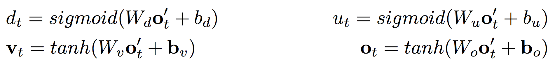
The high level takeaway of these formulas is that all of our inputs to the stack are conditioned on a vector called o_prime_t. If you are familiar with vanilla neural networks already, then this should be easy work. The code for these functions looks something like this.
import numpy as np

def sigmoid(x):
    return 1/(1+np.exp(-x))

def tanh(x):
    return np.tanh(x)

o_prime_dim = 5
stack_width = 2
output_dim = 3

o_prime_t = np.random.rand(o_prime_dim) # random input data

# weight matrix
W_d = np.random.rand(o_prime_dim,1) * 0.2 - 0.1
# bias
b_d = np.random.rand(1) * 0.2 - 0.1

# weight matrix
W_u = np.random.rand(o_prime_dim,1) * 0.2 - 0.1
# bias
b_u = np.random.rand(1) * 0.2 - 0.1

# weight matrix
W_v = np.random.rand(o_prime_dim,stack_width) * 0.2 - 0.1
#bias
b_v = np.random.rand(stack_width) * 0.2 - 0.1

#weight matrix
W_o = np.random.rand(o_prime_dim,output_dim) * 0.2 - 0.1
#bias
b_o = np.random.rand(output_dim) * 0.2 - 0.1

#forward propagation
d_t = sigmoid(np.dot(o_prime_t,W_d) + b_d)
u_t = sigmoid(np.dot(o_prime_t,W_u) + b_u)
v_t = tanh(np.dot(o_prime_t,W_v) + b_v)
o_t = tanh(np.dot(o_prime_t,W_o) + b_o)
So, this is another point where it would be tempting to hook up all of these controllers at once, build and RNN, and see if it converges. However, this is not wise. Instead, let's (again) just bite off the smallest piece that we can test. Let's start by just controlling u_t and d_t with a neural network by altering our previous codebase. This is also a good time to add some object oriented abstraction to our neural stack since we won't be changing it anymore (make it work... THEN make it pretty :) )
Note: I'm just writing the code inline for you to copy and run locally. This was getting a bit too computationally intense for a browser. I highly recommend downloading iPython Notebook and running all the rest of the examples in this blog in various notebooks. That's what I used to develop them. They're extremely effective for experimention and rapid prototyping.
import numpy as np
np.random.seed(1)

def sigmoid(x):
    return 1/(1+np.exp(-x))

def sigmoid_out2deriv(out):
    return out * (1 - out)

def tanh(x):
    return np.tanh(x)

def tanh_out2deriv(out):
    return (1 - out**2)

def relu(x,deriv=False):
    if(deriv):
        return int(x >= 0)
    return max(0,x)

class NeuralStack():
    def __init__(self,stack_width=2,o_prime_dim=6):
        self.stack_width = stack_width
        self.o_prime_dim = o_prime_dim
        self.reset()

    def reset(self):
        # INIT STACK
        self.V = list() # stack states
        self.s = list() # stack strengths
        self.d = list() # push strengths
        self.u = list() # pop strengths
        self.r = list()
        self.o = list()

        self.V_delta = list() # stack states
        self.s_delta = list() # stack strengths
        self.d_error = list() # push strengths
        self.u_error = list() # pop strengths

        self.t = 0

    def pushAndPopForward(self,v_t,d_t,u_t):

        self.d.append(d_t)
        self.d_error.append(0)

        self.u.append(u_t)
        self.u_error.append(0)

        new_s = np.zeros(self.t+1)
        for i in xrange(self.t+1):
            new_s[i] = self.s_t(i)
        self.s.append(new_s)
        self.s_delta.append(np.zeros_like(new_s))

        if(len(self.V) == 0):
            V_t = np.zeros((0,self.stack_width))
        else:
            V_t = self.V[-1]
        self.V.append(np.concatenate((V_t,np.atleast_2d(v_t)),axis=0))
        self.V_delta.append(np.zeros_like(self.V[-1]))

        r_t = self.r_t()
        self.r.append(r_t)

        self.t += 1
        return r_t

    def s_t(self,i):
        if(i >= 0 and i < self.t):
            inner_sum = self.s[self.t-1][i+1:self.t-0]
            return relu(self.s[self.t-1][i] - relu(self.u[self.t] - np.sum(inner_sum)))
        elif(i == self.t):
            return self.d[self.t]
        else:
            print "Problem"

    def s_t_error(self,i,error):
        if(i >= 0 and i < self.t):
            if(self.s_t(i) >= 0):
                self.s_delta[self.t-1][i] += error
                if(relu(self.u[self.t] - np.sum(self.s[self.t-1][i+1:self.t-0])) >= 0):
                    self.u_error[self.t] -= error
                    self.s_delta[self.t-1][i+1:self.t-0] += error
        elif(i == self.t):
            self.d_error[self.t] += error
        else:
            print "Problem"

    def r_t(self):
        r_t_out = np.zeros(self.stack_width)
        for i in xrange(0,self.t+1):
            temp = min(self.s[self.t][i],relu(1 - np.sum(self.s[self.t][i+1:self.t+1])))
            r_t_out += temp * self.V[self.t][i]
        return r_t_out

    def r_t_error(self,r_t_error):
        for i in xrange(0, self.t+1):
            temp = min(self.s[self.t][i],relu(1 - np.sum(self.s[self.t][i+1:self.t+1])))
            self.V_delta[self.t][i] += temp * r_t_error
            temp_error = np.sum(r_t_error * self.V[self.t][i])

            if(self.s[self.t][i] < relu(1 - np.sum(self.s[self.t][i+1:self.t+1]))):
                self.s_delta[self.t][i] += temp_error
            else:
                if(relu(1 - np.sum(self.s[self.t][i+1:self.t+1])) > 0):
                    self.s_delta[self.t][i+1:self.t+1] -= temp_error # minus equal becuase of the (1-).. and drop the 1

    def backprop(self,all_errors_in_order_of_training_data):
        errors = all_errors_in_order_of_training_data
        for error in reversed(list((errors))):
            self.t -= 1
            self.r_t_error(error)
            for i in reversed(xrange(self.t+1)):
                self.s_t_error(i,self.s_delta[self.t][i])


u_weights = np.array([0,0,0,0,0,0.0])

o_primes = np.eye(6)
y = np.array([1,0])
W_op_d = (np.random.randn(6,1) * 0.2) - 0.2
b_d = np.zeros(1)

W_op_u = (np.random.randn(6,1) * 0.2) - 0.2
b_u = np.zeros(1)

for h in xrange(10000):

    sequence = np.array([np.random.rand(3),[0,0,0]]).T
    sequence = np.concatenate((sequence,np.zeros_like(sequence)))

    stack = NeuralStack()

    d_weights = sigmoid(np.dot(o_primes,W_op_d) + b_d)
    u_weights = sigmoid(np.dot(o_primes,W_op_u) + b_u)

    reads = list()
    for i in xrange(6):
        reads.append(stack.pushAndPopForward(sequence[i],d_weights[i],u_weights[i]))

    reads = np.array(reads)

    reads[:3] *= 0 # eliminate errors we're not ready to backprop

    errors_in_order = reads - np.array(list(reversed(sequence)))

    stack.backprop(errors_in_order)

    # WEIGHT UPDATE
    alpha = 0.5

    u_delta = np.atleast_2d(np.array(stack.u_error) * sigmoid_out2deriv(u_weights)[0])
    W_op_u -= alpha * np.dot(o_primes,u_delta.T)
    b_u -= alpha * np.mean(u_delta)

    d_delta = np.atleast_2d(np.array(stack.d_error) * sigmoid_out2deriv(d_weights)[0])
    W_op_d -= alpha * np.dot(o_primes,d_delta.T)
    b_d -= alpha * np.mean(d_delta)

    for k in range(len(d_weights)):
        if d_weights[k] < 0:
            d_weights[k] = 0
        if u_weights[k] < 0:
            u_weights[k] = 0


    if(h % 100 == 0):
        print errors_in_order
Runtime Output:
[[ 0.          0.        ]
 [ 0.          0.        ]
 [ 0.          0.        ]
 [-0.79249511  0.        ]
 [-0.19810149  0.        ]
 [-0.14038694  0.        ]]

 .....
 .....
 .....

 [[ 0.          0.        ]
 [ 0.          0.        ]
 [ 0.          0.        ]
 [-0.00174623  0.        ]
 [ 0.0023387   0.        ]
 [-0.00084291  0.        ]]
Note that I'm logging errors this time instead of the discrete sequence.
All this code is doing is using two weight matrices W_op_u and W_op_d (and their biases) to predict u_t and d_t. We created mock o_prime_t variables to be different at each timestep. Instead of taking the delta at u_t and changing the u_weight directly. We used the delta at u_t to update the matrices W_op_u. Even though the code is cleaned up considerably, it's still doing the same thing for 99% of it.
Building Out The Rest of the Controller
So, all we're really doing now is taking the RNN from my previous blogpost on Recurrent Neural Networks and using it to generate o_prime_t. We then hook up the forward and backpropagation and we get the following code. I'm going to write the code in section here and describe (at a high level) what's going on. I'll then give you a single block with all the code together (that's runnable)
import numpy as np

def sigmoid(x):
    return 1/(1+np.exp(-x))

def sigmoid_out2deriv(out):
    return out * (1 - out)

def tanh(x):
    return np.tanh(x)

def tanh_out2deriv(out):
    return (1 - out**2)

def relu(x,deriv=False):
    if(deriv):
        return int(x >= 0)
    return max(0,x)
Seen this before. Just some utility nonlinearities to use at various layers. Note that I'm using relu here instead of using the "max(0,x)" from before. They are identical. So, wherever you used to see "max(0," you will now see "relu(".
class NeuralStack():
    def __init__(self,stack_width=2,o_prime_dim=6):
        self.stack_width = stack_width
        self.o_prime_dim = o_prime_dim
        self.reset()

    def reset(self):
        # INIT STACK
        self.V = list() # stack states
        self.s = list() # stack strengths
        self.d = list() # push strengths
        self.u = list() # pop strengths
        self.r = list()
        self.o = list()

        self.V_delta = list() # stack states
        self.s_delta = list() # stack strengths
        self.d_error = list() # push strengths
        self.u_error = list() # pop strengths

        self.t = 0

    def pushAndPopForward(self,v_t,d_t,u_t):

        self.d.append(d_t)
        self.d_error.append(0)

        self.u.append(u_t)
        self.u_error.append(0)

        new_s = np.zeros(self.t+1)
        for i in xrange(self.t+1):
            new_s[i] = self.s_t(i)
        self.s.append(new_s)
        self.s_delta.append(np.zeros_like(new_s))

        if(len(self.V) == 0):
            V_t = np.zeros((0,self.stack_width))
        else:
            V_t = self.V[-1]
        self.V.append(np.concatenate((V_t,np.atleast_2d(v_t)),axis=0))
        self.V_delta.append(np.zeros_like(self.V[-1]))

        r_t = self.r_t()
        self.r.append(r_t)

        self.t += 1
        return r_t

    def s_t(self,i):
        if(i >= 0 and i < self.t):
            inner_sum = self.s[self.t-1][i+1:self.t-0]
            return relu(self.s[self.t-1][i] - relu(self.u[self.t] - np.sum(inner_sum)))
        elif(i == self.t):
            return self.d[self.t]
        else:
            print "Problem"

    def s_t_error(self,i,error):
        if(i >= 0 and i < self.t):
            if(self.s_t(i) >= 0):
                self.s_delta[self.t-1][i] += error
                if(relu(self.u[self.t] - np.sum(self.s[self.t-1][i+1:self.t-0])) >= 0):
                    self.u_error[self.t] -= error
                    self.s_delta[self.t-1][i+1:self.t-0] += error
        elif(i == self.t):
            self.d_error[self.t] += error
        else:
            print "Problem"

    def r_t(self):
        r_t_out = np.zeros(self.stack_width)
        for i in xrange(0,self.t+1):
            temp = min(self.s[self.t][i],relu(1 - np.sum(self.s[self.t][i+1:self.t+1])))
            r_t_out += temp * self.V[self.t][i]
        return r_t_out

    def r_t_error(self,r_t_error):
        for i in xrange(0, self.t+1):
            temp = min(self.s[self.t][i],relu(1 - np.sum(self.s[self.t][i+1:self.t+1])))
            self.V_delta[self.t][i] += temp * r_t_error
            temp_error = np.sum(r_t_error * self.V[self.t][i])

            if(self.s[self.t][i] < relu(1 - np.sum(self.s[self.t][i+1:self.t+1]))):
                self.s_delta[self.t][i] += temp_error
            else:
                if(relu(1 - np.sum(self.s[self.t][i+1:self.t+1])) > 0):
                    self.s_delta[self.t][i+1:self.t+1] -= temp_error # minus equal becuase of the (1-).. and drop the 1
    def backprop_single(self,r_t_error):
        self.t -= 1
        self.r_t_error(r_t_error)
        for i in reversed(xrange(self.t+1)):
            self.s_t_error(i,self.s_delta[self.t][i])

    def backprop(self,all_errors_in_order_of_training_data):
        errors = all_errors_in_order_of_training_data
        for error in reversed(list((errors))):
            self.backprop_single(error)
This is pretty much the same Neural Stack we developed before. I broke the "backprop" method into two methods: backprop and backprop_single. Backpropagating over all the timesteps can be done by calling backprop. If you just want to backprop a single step at a time (which was useful when making sure to backprop through the RNN), then call backprop_single.
options = 2
sub_sequence_length = 2
sequence_length = sub_sequence_length*2

sequence = (np.random.random(sub_sequence_length)*options).astype(int)+1
sequence[-1] = 0
sequence

X = np.zeros((sub_sequence_length*2,options+1))
Y = np.zeros_like(X)
for i in xrange(len(sequence)):
    X[i][sequence[i]] = 1
    Y[-i][sequence[i]] = 1

x_dim = X.shape[1]
h_dim = 16
o_prime_dim = 16
stack_width = options
y_dim = Y.shape[1]
This segment of code does a couple things. First, it constructs a training example sequence. "sub_sequence_length" is the lengh of the sequence that we want to remember and then reverse with the neural stack. "options" is the number of unique elements in the sequence. Setting options to 2 generates a binary sequence, which is what we're running here. The sequence_length is just double the sub_sequence_length. This is because we need to first encode the whole sequence and then decode the whole sequence. So, if the sub_sequence_length is of length 5, then we have to generate 10 training examples (5 encoding and 5 decoding). Note that we set the last number in the sequence to 0 which is a special index indicating that we have reached the end of the sequence. The network will learn to start reversing at this point.
X and Y are our input and output training examples respectively. They one-hot encode our training data for both inputs and outputs.
Finally, we have the dimensionality of our neural network. In accordance with the paper, we the input dimension x_dim (equal to the number of "options" in our sequence plus one special character for the end of sequence marker). We also have two hidden layers. "h_dim" refers to the hidden layer in the recurrent neural network. "o_prime_dim" is the second hidden layer (generated from the recurrent hidden layer) which sends information into our neural stack. We have set the dimensionality of both hidden layers to 16. Note that this is WAY smaller than the 256 and 512 size layers in the paper. For ease, we're going to work with shorter binary sequences which require smaller hidden layers sizes (mostly because of the number of options, not the length of the sequence...)
"stack_width" is still the width of the vectors on the stack. In this case, I'm setting it to the number of options so that it can (in theory) one hot encode the input data into the stack. In theory you could actually use log_base_2(options) but this level of compression just requires more training time. I tried several experiments making this bigger with mixed results.
"y_dim" is the dimensionality of the output sequence to be predicted. Note that this could be (in theory) any sequence, but in this case it is the reverse of the input.
W_xh = (np.random.rand(x_dim,h_dim)*0.2) - 0.1
W_xh_update = np.zeros_like(W_xh)

W_hh = (np.random.rand(h_dim,h_dim)*0.2) - 0.1
W_hh_update = np.zeros_like(W_hh)

W_rh = (np.random.rand(stack_width,h_dim)*0.2) - 0.1
W_rh_update = np.zeros_like(W_rh)

b_h = (np.random.rand(h_dim)*0.2) - 0.1
b_h_update = np.zeros_like(b_h)

W_hop = (np.random.rand(h_dim,o_prime_dim) * 0.2) - 0.1
W_hop_update = np.zeros_like(W_hop)

b_op = (np.random.rand(o_prime_dim)*0.2) - 0.1
b_op_update = np.zeros_like(b_op)

W_op_d = (np.random.rand(o_prime_dim,1)*0.2) - 0.1
W_op_d_update = np.zeros_like(W_op_d)

W_op_u = (np.random.rand(o_prime_dim,1)*0.2) - 0.1
W_op_u_update = np.zeros_like(W_op_u)

W_op_v = (np.random.rand(o_prime_dim,stack_width)*0.2) - 0.1
W_op_v_update = np.zeros_like(W_op_v)

W_op_o = (np.random.rand(o_prime_dim,y_dim)*0.2) - 0.1
W_op_o_update = np.zeros_like(W_op_o)

b_d = (np.random.rand(1)*0.2)+0.1
b_d_update = np.zeros_like(b_d)

b_u = (np.random.rand(1)*0.2)-0.1
b_u_update = np.zeros_like(b_u)

b_v = (np.random.rand(stack_width)*0.2)-0.1
b_v_update = np.zeros_like(b_v)

b_o = (np.random.rand(y_dim)*0.2)-0.1
b_o_update = np.zeros_like(b_o)
This initializes all of our weight matrices necessary for the Recurrent Neural Network Controller. I generally used the notation W_ for weight matrices and b_ for biases. Following the W is shorthand for what it connects from and to. For example, W_xh connects the input (x) to the recurrent hidden layer (h). "op" is shorthand for "o_prime".
There is one other note here that you can find in the appendix of the paper. Initialization of b_d and b_u has significant impact on how well the neural stack is learned. In general, if the first iterations of the network don't push anything onto the stack, then no derivatives will backpropagate THROUGH the stack, and the neural network will just ignore it. Thus, initializing b_d (the push bias) to a higher number (+0.1 instead of -0.1) encourages the network to push onto the neural stack during the beginning of training. This has a nice parallel intuition to life. If you had a stack but never pushed anything onto it... how would you know what it does? Generally the same thing going on here intuitively.
The reason we have _update variables is that we're going to be implementing mini-batch updates. Thus, we'll create updates and save them in the _update variables and only occasionally update the actual variables. This make for smoother training. See more on this in previous blogposts.
error = 0
max_len = 1
batch_size = 10
for it in xrange(1000000000):

    sub_sequence_length = np.random.randint(max_len)+1
    sequence = (np.random.random(sub_sequence_length)*options).astype(int)+1
#     sequence[-1] = 0
    sequence

    X = np.zeros((sub_sequence_length*2,options+1))
    Y = np.zeros_like(X)
    for i in xrange(len(sequence)):
        X[i][sequence[i]] = 1
        X[i][0] = 1
        Y[-i-1][sequence[i]] = 1
Ok, so the logic above that creates training examples doesn't exactly get used. I just use that section further up to experiment with the training example logic. I encourage you to do it. As you can see here, we randomly generate new training examples as we go. Note that "max_len" refers to the maximum length that we will model initially. As the error goes down (the neural network learns), this number will increase, modeling longer and longer sequences. Basically, we start by training the neural stack on short sequences, and once it gets good at those we start presenting longer ones. Experimenting with how long to start with was very fascinating to me. I highly encourage playing around with it.
layers = list()
stack = NeuralStack(stack_width=stack_width,o_prime_dim=o_prime_dim)
for i in xrange(len(X)):
    layer = {}

    layer['x'] = X[i]

    if(i == 0):
        layer['h_t-1'] = np.zeros(h_dim)
        layer['h_t-1'][0] = 1
        layer['r_t-1'] = np.zeros(stack_width)
        layer['r_t-1'][0] = 1
    else:
        layer['h_t-1'] = layers[i-1]['h_t']
        layer['r_t-1'] = layers[i-1]['r_t']

    layer['h_t'] = tanh(np.dot(layer['x'],W_xh) + np.dot(layer['h_t-1'],W_hh) + np.dot(layer['r_t-1'],W_rh) + b_h)
    layer['o_prime_t'] = tanh(np.dot(layer['h_t'],W_hop)+b_op)
    layer['o_t'] = tanh(np.dot(layer['o_prime_t'],W_op_o) + b_o)

    if(i < len(X)-1):
        layer['d_t'] = sigmoid(np.dot(layer['o_prime_t'],W_op_d) + b_d)
        layer['u_t'] = sigmoid(np.dot(layer['o_prime_t'],W_op_u) + b_u)
        layer['v_t'] = tanh(np.dot(layer['o_prime_t'],W_op_v) + b_v)

        layer['r_t'] = stack.pushAndPopForward(layer['v_t'],layer['d_t'],layer['u_t'])

    layers.append(layer)
This is the forward propagation step. Notice that it's just a recurrent neural network with one extra input r_t-1 which is the neural stack r_t from the previous timestep. Generally, you can also see that x->h, h->o_prime, o_prime->stack_controllers, stack_controllers->stack, stack->r_t, and then r_t is fed into the next layer. Study this portion of code until the "information flow" becomes clear. Also notice the convention I use of storing the intermediate variables into the "layers" list. This will help make backpropagation easier later. Note that the prediction of the neural network is layer['o'] which isn't exactly what we read off of the stack. Information must travel from the stack to the hidden layer and out through layer['o']. We'll talk more about how to encourage this in a minute.
for i in list(reversed(xrange(len(X)))):
    layer = layers[i]

    layer['o_t_error'] = Y[i] - layer['o_t']
    error += np.sum(np.abs(layer['o_t_error']))
    if(it % 100 == 99):
        if(i == len(X)-1):
            if(it % 10000 == 9999):
                print "MaxLen:"+str(max_len)+ " Iter:" + str(it) + " Error:" + str(error) + "True:" + str(sequence) + " Pred:" + str(map(lambda x:np.argmax(x['o_t']),layers[sub_sequence_length:]))
            if(error < (5*max_len)):
                max_len+=1
            error = 0

#                     sub_sequence_length += 1
#             print str(Y[i]) + " - " + str(layer['o_t']) + " = " + str(layer['o_t_error'])
    layer['o_t_delta'] = layer['o_t_error'] * tanh_out2deriv(layer['o_t'])

    layer['o_prime_t_error'] = np.dot(layer['o_t_delta'],W_op_o.T)

    if(i < len(X)-1):
        layer['r_t_error'] = layers[i+1]['r_t-1_error']
        stack.backprop_single(layer['r_t_error'])

        layer['v_t_error'] = stack.V_delta[i][i]
        layer['v_t_delta'] = layer['v_t_error'] * tanh_out2deriv(layer['v_t'])
        layer['o_prime_t_error'] += np.dot(layer['v_t_delta'],W_op_v.T)

        layer['u_t_error'] = stack.u_error[i]
        layer['u_t_delta'] = layer['u_t_error'] * sigmoid_out2deriv(layer['u_t'])
        layer['o_prime_t_error'] += np.dot(layer['u_t_delta'],W_op_u.T)

        layer['d_t_error'] = stack.d_error[i]
        layer['d_t_delta'] = layer['d_t_error'] * sigmoid_out2deriv(layer['d_t'])
        layer['o_prime_t_error'] += np.dot(layer['d_t_delta'],W_op_d.T)


    layer['o_prime_t_delta'] = layer['o_prime_t_error'] * tanh_out2deriv(layer['o_prime_t'])
    layer['h_t_error'] = np.dot(layer['o_prime_t_delta'],W_hop.T)

    if(i < len(X)-1):
        layer['h_t_error'] += layers[i+1]['h_t-1_error']

    layer['h_t_delta'] = layer['h_t_error'] * tanh_out2deriv(layer['h_t'])
    layer['h_t-1_error'] = np.dot(layer['h_t_delta'],W_hh.T)
    layer['r_t-1_error'] = np.dot(layer['h_t_delta'],W_rh.T)
This is the backpropagation step. Again, we're just taking the delta we get from the neural stack and then backpropagating it through all the layers just like we did with the recurrent neural network in the previous blogpost. Also note the logic on lines 7-13. If the error gets below 5*max_len, then it increases the length of the sequence it's trying to model by 1 at the next iteration.
for i in xrange(len(X)):
    layer = layers[i]
    max_alpha = 0.005 * batch_size
    alpha = max_alpha / sub_sequence_length

    W_xh_update += alpha * np.outer(layer['x'],layer['h_t_delta'])
    W_hh_update += alpha * np.outer(layer['h_t-1'],layer['h_t_delta'])
    W_rh_update += alpha * np.outer(layer['r_t-1'],layer['h_t_delta'])
    b_h_update += alpha * layer['h_t_delta']

    W_hop_update += alpha * np.outer(layer['h_t'],layer['o_prime_t_delta'])
    b_op_update += alpha * layer['o_prime_t_delta']

    if(i < len(X)-1):
        W_op_d_update += alpha * np.outer(layer['o_prime_t'],layer['d_t_delta'])
        W_op_u_update += alpha * np.outer(layer['o_prime_t'],layer['u_t_delta'])
        W_op_v_update += alpha * np.outer(layer['o_prime_t'],layer['v_t_delta'])

        b_d_update += alpha * layer['d_t_delta']
        b_u_update += alpha * layer['u_t_delta']
        b_v_update += alpha * layer['v_t_delta']

    W_op_o_update += alpha * np.outer(layer['o_prime_t'],layer['o_t_delta'])
    b_o_update += alpha * layer['o_t_delta']
At this phase, we create our weight updates by multiplying the outer product of each layers weights by the deltas at the immediately following layer. We save these updates aside into our _update variables. Note that this doesn't change the weights. It just collects the updates.
if(it % batch_size == (batch_size-1)):
    W_xh += W_xh_update/batch_size
    W_xh_update *= 0

    W_hh += W_hh_update/batch_size
    W_hh_update *= 0

    W_rh += W_rh_update/batch_size
    W_rh_update *= 0

    b_h += b_h_update/batch_size
    b_h_update *= 0

    W_hop += W_hop_update/batch_size
    W_hop_update *= 0

    b_op += b_op_update/batch_size
    b_op_update *= 0

    W_op_d += W_op_d_update/batch_size
    W_op_d_update *= 0

    W_op_u += W_op_u_update/batch_size
    W_op_u_update *= 0

    W_op_v += W_op_v_update/batch_size
    W_op_v_update *= 0

    b_d += b_d_update/batch_size
    b_d_update *= 0

    b_d += b_d * 0.00025 * batch_size
    b_u += b_u_update/batch_size
    b_u_update *= 0

    b_v += b_v_update/batch_size
    b_v_update *= 0

    W_op_o += W_op_o_update/batch_size
    W_op_o_update *= 0

    b_o += b_o_update/batch_size
    b_o_update *= 0
And if we are at the end of a mini-batch, then we update the weights using the average of all the updates we had accumulated so far. We then clear out each _update variable by multiplying it by 0.
And We Have It!!!
So, for all the code in one big file for you to run
import numpy as np

def sigmoid(x):
    return 1/(1+np.exp(-x))

def sigmoid_out2deriv(out):
    return out * (1 - out)

def tanh(x):
    return np.tanh(x)

def tanh_out2deriv(out):
    return (1 - out**2)

def relu(x,deriv=False):
    if(deriv):
        return int(x >= 0)
    return max(0,x)

class NeuralStack():
    def __init__(self,stack_width=2,o_prime_dim=6):
        self.stack_width = stack_width
        self.o_prime_dim = o_prime_dim
        self.reset()

    def reset(self):
        # INIT STACK
        self.V = list() # stack states
        self.s = list() # stack strengths
        self.d = list() # push strengths
        self.u = list() # pop strengths
        self.r = list()
        self.o = list()

        self.V_delta = list() # stack states
        self.s_delta = list() # stack strengths
        self.d_error = list() # push strengths
        self.u_error = list() # pop strengths

        self.t = 0

    def pushAndPopForward(self,v_t,d_t,u_t):

        self.d.append(d_t)
        self.d_error.append(0)

        self.u.append(u_t)
        self.u_error.append(0)

        new_s = np.zeros(self.t+1)
        for i in xrange(self.t+1):
            new_s[i] = self.s_t(i)
        self.s.append(new_s)
        self.s_delta.append(np.zeros_like(new_s))

        if(len(self.V) == 0):
            V_t = np.zeros((0,self.stack_width))
        else:
            V_t = self.V[-1]
        self.V.append(np.concatenate((V_t,np.atleast_2d(v_t)),axis=0))
        self.V_delta.append(np.zeros_like(self.V[-1]))

        r_t = self.r_t()
        self.r.append(r_t)

        self.t += 1
        return r_t

    def s_t(self,i):
        if(i >= 0 and i < self.t):
            inner_sum = self.s[self.t-1][i+1:self.t-0]
            return relu(self.s[self.t-1][i] - relu(self.u[self.t] - np.sum(inner_sum)))
        elif(i == self.t):
            return self.d[self.t]
        else:
            print "Problem"

    def s_t_error(self,i,error):
        if(i >= 0 and i < self.t):
            if(self.s_t(i) >= 0):
                self.s_delta[self.t-1][i] += error
                if(relu(self.u[self.t] - np.sum(self.s[self.t-1][i+1:self.t-0])) >= 0):
                    self.u_error[self.t] -= error
                    self.s_delta[self.t-1][i+1:self.t-0] += error
        elif(i == self.t):
            self.d_error[self.t] += error
        else:
            print "Problem"

    def r_t(self):
        r_t_out = np.zeros(self.stack_width)
        for i in xrange(0,self.t+1):
            temp = min(self.s[self.t][i],relu(1 - np.sum(self.s[self.t][i+1:self.t+1])))
            r_t_out += temp * self.V[self.t][i]
        return r_t_out

    def r_t_error(self,r_t_error):
        for i in xrange(0, self.t+1):
            temp = min(self.s[self.t][i],relu(1 - np.sum(self.s[self.t][i+1:self.t+1])))
            self.V_delta[self.t][i] += temp * r_t_error
            temp_error = np.sum(r_t_error * self.V[self.t][i])

            if(self.s[self.t][i] < relu(1 - np.sum(self.s[self.t][i+1:self.t+1]))):
                self.s_delta[self.t][i] += temp_error
            else:
                if(relu(1 - np.sum(self.s[self.t][i+1:self.t+1])) > 0):
                    self.s_delta[self.t][i+1:self.t+1] -= temp_error # minus equal becuase of the (1-).. and drop the 1
    def backprop_single(self,r_t_error):
        self.t -= 1
        self.r_t_error(r_t_error)
        for i in reversed(xrange(self.t+1)):
            self.s_t_error(i,self.s_delta[self.t][i])

    def backprop(self,all_errors_in_order_of_training_data):
        errors = all_errors_in_order_of_training_data
        for error in reversed(list((errors))):
            self.backprop_single(error)


options = 2
sub_sequence_length = 5
sequence_length = sub_sequence_length*2

sequence = (np.random.random(sub_sequence_length)*options).astype(int)+1
sequence[-1] = 0
sequence

X = np.zeros((sub_sequence_length*2,options+1))
Y = np.zeros_like(X)
for i in xrange(len(sequence)):
    X[i][sequence[i]] = 1
    Y[-i][sequence[i]] = 1

sequence_length = len(X)
x_dim = X.shape[1]
h_dim = 16
o_prime_dim = 16
stack_width = options
y_dim = Y.shape[1]


sub_sequence_length = 2

W_xh = (np.random.rand(x_dim,h_dim)*0.2) - 0.1
W_xh_update = np.zeros_like(W_xh)

W_hh = (np.random.rand(h_dim,h_dim)*0.2) - 0.1
W_hh_update = np.zeros_like(W_hh)

W_rh = (np.random.rand(stack_width,h_dim)*0.2) - 0.1
W_rh_update = np.zeros_like(W_rh)

b_h = (np.random.rand(h_dim)*0.2) - 0.1
b_h_update = np.zeros_like(b_h)

W_hop = (np.random.rand(h_dim,o_prime_dim) * 0.2) - 0.1
W_hop_update = np.zeros_like(W_hop)

b_op = (np.random.rand(o_prime_dim)*0.2) - 0.1
b_op_update = np.zeros_like(b_op)

W_op_d = (np.random.rand(o_prime_dim,1)*0.2) - 0.1
W_op_d_update = np.zeros_like(W_op_d)

W_op_u = (np.random.rand(o_prime_dim,1)*0.2) - 0.1
W_op_u_update = np.zeros_like(W_op_u)

W_op_v = (np.random.rand(o_prime_dim,stack_width)*0.2) - 0.1
W_op_v_update = np.zeros_like(W_op_v)

W_op_o = (np.random.rand(o_prime_dim,y_dim)*0.2) - 0.1
W_op_o_update = np.zeros_like(W_op_o)

b_d = (np.random.rand(1)*0.2)+0.1
b_d_update = np.zeros_like(b_d)

b_u = (np.random.rand(1)*0.2)-0.1
b_u_update = np.zeros_like(b_u)

b_v = (np.random.rand(stack_width)*0.2)-0.1
b_v_update = np.zeros_like(b_v)

b_o = (np.random.rand(y_dim)*0.2)-0.1
b_o_update = np.zeros_like(b_o)

error = 0
max_len = 1
batch_size = 10
for it in xrange(1000000000):

    sub_sequence_length = np.random.randint(max_len)+1
    sequence = (np.random.random(sub_sequence_length)*options).astype(int)+1
#     sequence[-1] = 0
    sequence

    X = np.zeros((sub_sequence_length*2,options+1))
    Y = np.zeros_like(X)
    for i in xrange(len(sequence)):
        X[i][sequence[i]] = 1
        X[i][0] = 1
        Y[-i-1][sequence[i]] = 1

    layers = list()
    stack = NeuralStack(stack_width=stack_width,o_prime_dim=o_prime_dim)
    for i in xrange(len(X)):
        layer = {}

        layer['x'] = X[i]

        if(i == 0):
            layer['h_t-1'] = np.zeros(h_dim)
            layer['h_t-1'][0] = 1
            layer['r_t-1'] = np.zeros(stack_width)
            layer['r_t-1'][0] = 1
        else:
            layer['h_t-1'] = layers[i-1]['h_t']
            layer['r_t-1'] = layers[i-1]['r_t']

        layer['h_t'] = tanh(np.dot(layer['x'],W_xh) + np.dot(layer['h_t-1'],W_hh) + np.dot(layer['r_t-1'],W_rh) + b_h)
        layer['o_prime_t'] = tanh(np.dot(layer['h_t'],W_hop)+b_op)
        layer['o_t'] = tanh(np.dot(layer['o_prime_t'],W_op_o) + b_o)

        if(i < len(X)-1):
            layer['d_t'] = sigmoid(np.dot(layer['o_prime_t'],W_op_d) + b_d)
            layer['u_t'] = sigmoid(np.dot(layer['o_prime_t'],W_op_u) + b_u)
            layer['v_t'] = tanh(np.dot(layer['o_prime_t'],W_op_v) + b_v)

            layer['r_t'] = stack.pushAndPopForward(layer['v_t'],layer['d_t'],layer['u_t'])

        layers.append(layer)

    for i in list(reversed(xrange(len(X)))):
        layer = layers[i]

        layer['o_t_error'] = Y[i] - layer['o_t']
        error += np.sum(np.abs(layer['o_t_error']))
        if(it % 100 == 99):
            if(i == len(X)-1):
                if(it % 10000 == 9999):
                    print "MaxLen:"+str(max_len)+ " Iter:" + str(it) + " Error:" + str(error) + "True:" + str(sequence) + " Pred:" + str(map(lambda x:np.argmax(x['o_t']),layers[sub_sequence_length:]))
                if(error < (5*max_len)):
                    max_len+=1
                error = 0

        layer['o_t_delta'] = layer['o_t_error'] * tanh_out2deriv(layer['o_t'])

        layer['o_prime_t_error'] = np.dot(layer['o_t_delta'],W_op_o.T)

        if(i < len(X)-1):
            layer['r_t_error'] = layers[i+1]['r_t-1_error']
            stack.backprop_single(layer['r_t_error'])

            layer['v_t_error'] = stack.V_delta[i][i]
            layer['v_t_delta'] = layer['v_t_error'] * tanh_out2deriv(layer['v_t'])
            layer['o_prime_t_error'] += np.dot(layer['v_t_delta'],W_op_v.T)

            layer['u_t_error'] = stack.u_error[i]
            layer['u_t_delta'] = layer['u_t_error'] * sigmoid_out2deriv(layer['u_t'])
            layer['o_prime_t_error'] += np.dot(layer['u_t_delta'],W_op_u.T)

            layer['d_t_error'] = stack.d_error[i]
            layer['d_t_delta'] = layer['d_t_error'] * sigmoid_out2deriv(layer['d_t'])
            layer['o_prime_t_error'] += np.dot(layer['d_t_delta'],W_op_d.T)


        layer['o_prime_t_delta'] = layer['o_prime_t_error'] * tanh_out2deriv(layer['o_prime_t'])
        layer['h_t_error'] = np.dot(layer['o_prime_t_delta'],W_hop.T)

        if(i < len(X)-1):
            layer['h_t_error'] += layers[i+1]['h_t-1_error']

        layer['h_t_delta'] = layer['h_t_error'] * tanh_out2deriv(layer['h_t'])
        layer['h_t-1_error'] = np.dot(layer['h_t_delta'],W_hh.T)
        layer['r_t-1_error'] = np.dot(layer['h_t_delta'],W_rh.T)

    for i in xrange(len(X)):
        layer = layers[i]
        max_alpha = 0.005 * batch_size
        alpha = max_alpha / sub_sequence_length

        W_xh_update += alpha * np.outer(layer['x'],layer['h_t_delta'])
        W_hh_update += alpha * np.outer(layer['h_t-1'],layer['h_t_delta'])
        W_rh_update += alpha * np.outer(layer['r_t-1'],layer['h_t_delta'])
        b_h_update += alpha * layer['h_t_delta']

        W_hop_update += alpha * np.outer(layer['h_t'],layer['o_prime_t_delta'])
        b_op_update += alpha * layer['o_prime_t_delta']

        if(i < len(X)-1):
            W_op_d_update += alpha * np.outer(layer['o_prime_t'],layer['d_t_delta'])
            W_op_u_update += alpha * np.outer(layer['o_prime_t'],layer['u_t_delta'])
            W_op_v_update += alpha * np.outer(layer['o_prime_t'],layer['v_t_delta'])

            b_d_update += alpha * layer['d_t_delta']
            b_u_update += alpha * layer['u_t_delta']
            b_v_update += alpha * layer['v_t_delta']

        W_op_o_update += alpha * np.outer(layer['o_prime_t'],layer['o_t_delta'])
        b_o_update += alpha * layer['o_t_delta']


    if(it % batch_size == (batch_size-1)):
        W_xh += W_xh_update/batch_size
        W_xh_update *= 0

        W_hh += W_hh_update/batch_size
        W_hh_update *= 0

        W_rh += W_rh_update/batch_size
        W_rh_update *= 0

        b_h += b_h_update/batch_size
        b_h_update *= 0

        W_hop += W_hop_update/batch_size
        W_hop_update *= 0

        b_op += b_op_update/batch_size
        b_op_update *= 0

        W_op_d += W_op_d_update/batch_size
        W_op_d_update *= 0

        W_op_u += W_op_u_update/batch_size
        W_op_u_update *= 0

        W_op_v += W_op_v_update/batch_size
        W_op_v_update *= 0

        b_d += b_d_update/batch_size
        b_d_update *= 0

        b_d += b_d * 0.00025 * batch_size
        b_u += b_u_update/batch_size
        b_u_update *= 0

        b_v += b_v_update/batch_size
        b_v_update *= 0

        W_op_o += W_op_o_update/batch_size
        W_op_o_update *= 0

        b_o += b_o_update/batch_size
        b_o_update *= 0
Expected Output:
If you run this code overnight on your CPU...you should see output that looks a lot like this. Note that the predictions are the reverse of the original sequence.
.......
.......
.......
.......
MaxLen:19 Iter:2789999 Error:168.444794145True:[2 2 1 1 2 1 2 1 1 2] Pred:[2, 1, 1, 2, 1, 2, 1, 1, 2, 2]
MaxLen:19 Iter:2799999 Error:207.262352698True:[1] Pred:[1]
MaxLen:19 Iter:2809999 Error:182.105266119True:[1 1 2 1 2 2 2 1 1 2 1] Pred:[1, 2, 1, 1, 2, 2, 2, 1, 2, 1, 1]
MaxLen:19 Iter:2819999 Error:184.174791858True:[2 1 2 2] Pred:[2, 2, 1, 2]
MaxLen:19 Iter:2829999 Error:206.158101496True:[2 1 2 2 2 1 1 2] Pred:[2, 1, 1, 2, 2, 2, 1, 2]
MaxLen:19 Iter:2839999 Error:209.114103766True:[1 2 1 2 2 2 1 1 1 1 2] Pred:[2, 1, 1, 1, 1, 2, 2, 2, 1, 2, 1]
MaxLen:19 Iter:2849999 Error:167.128615254True:[2 1 2 1 1 2 1 2 1 2 1 1 2 2 2 1 2] Pred:[2, 1, 2, 2, 2, 1, 2, 2, 1, 2, 1, 2, 1, 1, 2, 1, 2]
MaxLen:19 Iter:2859999 Error:200.380921774True:[2 2 2 1 1] Pred:[1, 1, 2, 2, 2]
MaxLen:19 Iter:2869999 Error:112.94541202True:[2 2 1 2 2 1 2 2 1 1 2 1 2] Pred:[2, 1, 2, 1, 1, 2, 2, 1, 2, 2, 1, 2, 2]
MaxLen:19 Iter:2879999 Error:160.091183839True:[2 1 2 2 1 2] Pred:[2, 1, 2, 2, 1, 2]
MaxLen:19 Iter:2889999 Error:112.598129039True:[1 1 2] Pred:[2, 1, 1]
MaxLen:19 Iter:2899999 Error:186.041933391True:[2 2 2 1 1 2 1 2 2 1 1 2 2 1] Pred:[1, 2, 2, 1, 1, 2, 2, 1, 2, 1, 1, 2, 2, 2]
MaxLen:19 Iter:2909999 Error:236.064449725True:[2 2 2 1 1 2 2 1 2 2 1 1 1 1 1 2 2] Pred:[2, 2, 1, 1, 1, 1, 1, 2, 1, 1, 2, 2, 1, 1, 2, 2, 1]
MaxLen:19 Iter:2919999 Error:152.776428031True:[1 1 2 1 1 1 1 2 2 1 1 1 2 2 1 2 2] Pred:[2, 2, 1, 2, 2, 1, 1, 1, 2, 2, 1, 1, 1, 1, 1, 1, 2]
MaxLen:19 Iter:2929999 Error:143.007796452True:[1 2 1 1] Pred:[1, 1, 2, 1]
MaxLen:19 Iter:2939999 Error:255.744221264True:[2 2 1 1 1 2 1] Pred:[1, 2, 1, 1, 1, 2, 2]
MaxLen:19 Iter:2949999 Error:183.147078344True:[1 2 1 1 2 2 1 1 1 1 2 1 1 1 2 1] Pred:[1, 2, 1, 1, 1, 2, 1, 1, 1, 1, 2, 2, 1, 1, 2, 2]
MaxLen:19 Iter:2959999 Error:231.447857024True:[2 2 1 1] Pred:[1, 1, 2, 2]
Something Went Wrong!!!
At this point, I declared victory! I broke open a few brewskis and kicked back. Yay! Deepmind's Neural Stack before my very eyes! How bout it! Alas... I started taking things apart and realized that something was wrong... most notably these two things. Immediately after this log ending I printed out the following variables.
stack.u
[array([ 0.52627134]),
 array([ 0.48875265]),
 array([ 0.4833596]),
 array([ 0.51072936]),
 array([ 0.51525512]),
 array([ 0.55418935]),
 array([ 0.51561233]),
 array([ 0.54271031]),
 array([ 0.46972942]),
 array([ 0.50030726]),
 array([ 0.50420808]),
 array([ 0.51277284]),
 array([ 0.49249017]),
 array([ 0.52770061]),
 array([ 0.53647627]),
 array([ 0.52879516]),
 array([ 0.57190229]),
 array([ 0.51895631]),
 array([ 0.50232574]),
 array([ 0.44804661]),
 array([ 0.50789469]),
 array([ 0.53620111]),
 array([ 0.57897974]),
 array([ 0.53155877])]
satck.d
[array([ 1.]),
 array([ 1.]),
 array([ 1.]),
 array([ 1.]),
 array([ 1.]),
 array([ 1.]),
 array([ 1.]),
 array([ 1.]),
 array([ 1.]),
 array([ 1.]),
 array([ 1.]),
 array([ 1.]),
 array([ 1.]),
 array([ 1.]),
 array([ 1.]),
 array([ 1.]),
 array([ 1.]),
 array([ 1.]),
 array([ 1.]),
 array([ 1.]),
 array([ 1.]),
 array([ 1.]),
 array([ 1.]),
 array([ 1.])]
Disaster... the neural network somehow learned how to model these sequences by pushing all of them onto the stack and then only popping off each number half at a time. What does this mean? Honestly, it could certainly be that I didn't train long enough. What do we do? Andrew... why are you sharing this with us? Was this 30 pages of blogging all for nothing?!?!
At this point, we have reached a very realistic point in a neural network researcher's lifecycle. Furthermore, it's one that the authors have discussed somewhat extensively both in the paper and in external presentations. If we're not careful, the network can discover less than expected ways of solving the problem that you give it. So, what do we do?
Part 6: When Things Really Get Interesting
I did end up getting the neural network to push and pop correctly. Here's the code. This blog is already like 80 pages long on my laptop so... Enjoy the puzzle!
Hint: Autoencoder
import numpy as np

def sigmoid(x):
    return 1/(1+np.exp(-x))

def sigmoid_out2deriv(out):
    return out * (1 - out)

def tanh(x):
    return np.tanh(x)

def tanh_out2deriv(out):
    return (1 - out**2)

def relu(x,deriv=False):
    if(deriv):
        return int(x >= 0)
    return max(0,x)

class NeuralStack():
    def __init__(self,stack_width=2,o_prime_dim=6):
        self.stack_width = stack_width
        self.o_prime_dim = o_prime_dim
        self.reset()

    def reset(self):
        # INIT STACK
        self.V = list() # stack states
        self.s = list() # stack strengths
        self.d = list() # push strengths
        self.u = list() # pop strengths
        self.r = list()
        self.o = list()

        self.V_delta = list() # stack states
        self.s_delta = list() # stack strengths
        self.d_error = list() # push strengths
        self.u_error = list() # pop strengths

        self.t = 0

    def pushAndPopForward(self,v_t,d_t,u_t):

        self.d.append(d_t)
        self.d_error.append(0)

        self.u.append(u_t)
        self.u_error.append(0)

        new_s = np.zeros(self.t+1)
        for i in xrange(self.t+1):
            new_s[i] = self.s_t(i)
        self.s.append(new_s)
        self.s_delta.append(np.zeros_like(new_s))

        if(len(self.V) == 0):
            V_t = np.zeros((0,self.stack_width))
        else:
            V_t = self.V[-1]
        self.V.append(np.concatenate((V_t,np.atleast_2d(v_t)),axis=0))
        self.V_delta.append(np.zeros_like(self.V[-1]))

        r_t = self.r_t()
        self.r.append(r_t)

        self.t += 1
        return r_t

    def s_t(self,i):
        if(i >= 0 and i < self.t):
            inner_sum = self.s[self.t-1][i+1:self.t-0]
            return relu(self.s[self.t-1][i] - relu(self.u[self.t] - np.sum(inner_sum)))
        elif(i == self.t):
            return self.d[self.t]
        else:
            print "Problem"

    def s_t_error(self,i,error):
        if(i >= 0 and i < self.t):
            if(self.s_t(i) >= 0):
                self.s_delta[self.t-1][i] += error
                if(relu(self.u[self.t] - np.sum(self.s[self.t-1][i+1:self.t-0])) >= 0):
                    self.u_error[self.t] -= error
                    self.s_delta[self.t-1][i+1:self.t-0] += error
        elif(i == self.t):
            self.d_error[self.t] += error
        else:
            print "Problem"

    def r_t(self):
        r_t_out = np.zeros(self.stack_width)
        for i in xrange(0,self.t+1):
            temp = min(self.s[self.t][i],relu(1 - np.sum(self.s[self.t][i+1:self.t+1])))
            r_t_out += temp * self.V[self.t][i]
        return r_t_out

    def r_t_error(self,r_t_error):
        for i in xrange(0, self.t+1):
            temp = min(self.s[self.t][i],relu(1 - np.sum(self.s[self.t][i+1:self.t+1])))
            self.V_delta[self.t][i] += temp * r_t_error
            temp_error = np.sum(r_t_error * self.V[self.t][i])

            if(self.s[self.t][i] < relu(1 - np.sum(self.s[self.t][i+1:self.t+1]))):
                self.s_delta[self.t][i] += temp_error
            else:
                if(relu(1 - np.sum(self.s[self.t][i+1:self.t+1])) > 0):
                    self.s_delta[self.t][i+1:self.t+1] -= temp_error # minus equal becuase of the (1-).. and drop the 1
    def backprop_single(self,r_t_error):
        self.t -= 1
        self.r_t_error(r_t_error)
        for i in reversed(xrange(self.t+1)):
            self.s_t_error(i,self.s_delta[self.t][i])

    def backprop(self,all_errors_in_order_of_training_data):
        errors = all_errors_in_order_of_training_data
        for error in reversed(list((errors))):
            self.backprop_single(error)


options = 2
sub_sequence_length = 5
sequence_length = sub_sequence_length*2

sequence = (np.random.random(sub_sequence_length)*options).astype(int)+2
sequence

X = np.zeros((sub_sequence_length*2,options+2))
Y = np.zeros_like(X)
for i in xrange(len(sequence)):
    X[i][sequence[i]] = 1
    X[-i-1][0] = 1
    X[i][1] = 1
    Y[-i-1][sequence[i]] = 1

sequence_length = len(X)
x_dim = X.shape[1]
h_dim = 8
o_prime_dim = 8
stack_width = 2
y_dim = Y.shape[1]


np.random.seed(1)
sub_sequence_length = 2

W_xh = (np.random.rand(x_dim,h_dim)*0.2) - 0.1
W_xh_update = np.zeros_like(W_xh)

W_hox = (np.random.rand(h_dim,x_dim)*0.2) - 0.1
W_hox_update = np.zeros_like(W_hox)

W_opx = (np.random.rand(o_prime_dim,x_dim)*0.2) - 0.1
W_opx_update = np.zeros_like(W_opx)

W_hh = (np.random.rand(h_dim,h_dim)*0.2) - 0.1
W_hh_update = np.zeros_like(W_hh)

W_rh = (np.random.rand(stack_width,h_dim)*0.2) - 0.1
W_rh_update = np.zeros_like(W_rh)

b_h = (np.random.rand(h_dim)*0.2) - 0.1
b_h_update = np.zeros_like(b_h)

W_hop = (np.random.rand(h_dim,o_prime_dim) * 0.2) - 0.1
W_hop_update = np.zeros_like(W_hop)

b_op = (np.random.rand(o_prime_dim)*0.2) - 0.1
b_op_update = np.zeros_like(b_op)

W_op_d = (np.random.rand(o_prime_dim,1)*0.2) - 0.1
W_op_d_update = np.zeros_like(W_op_d)

W_op_u = (np.random.rand(o_prime_dim,1)*0.2) - 0.1
W_op_u_update = np.zeros_like(W_op_u)

W_op_v = (np.random.rand(o_prime_dim,stack_width)*0.2) - 0.1
W_op_v_update = np.zeros_like(W_op_v)

W_op_o = (np.random.rand(o_prime_dim,y_dim)*0.2) - 0.1
W_op_o_update = np.zeros_like(W_op_o)

b_d = (np.random.rand(1)*0.2)+1
b_d_update = np.zeros_like(b_d)

b_u = (np.random.rand(1)*0.2)-1
b_u_update = np.zeros_like(b_u)

b_v = (np.random.rand(stack_width)*0.2)-0.1
b_v_update = np.zeros_like(b_v)

b_o = (np.random.rand(y_dim)*0.2)-0.1
b_o_update = np.zeros_like(b_o)

error = 0
reconstruct_error = 0
reconstruct_error_2 = 0
max_len = 3
batch_size = 50
for it in xrange(750000):

#     if(it % 100 == 0):
    sub_sequence_length = np.random.randint(max_len)+3
    sequence = (np.random.random(sub_sequence_length)*options).astype(int)+2
    sequence

    X = np.zeros((sub_sequence_length*2,options+2))
    Y = np.zeros_like(X)
    for i in xrange(len(sequence)):
        X[i][sequence[i]] = 1
        X[-i-1][0] = 1
        X[i][1] = 1
        Y[-i-1][sequence[i]] = 1


    layers = list()
    stack = NeuralStack(stack_width=stack_width,o_prime_dim=o_prime_dim)
    for i in xrange(len(X)):
        layer = {}

        layer['x'] = X[i]

        if(i == 0):
            layer['h_t-1'] = np.zeros(h_dim)
#             layer['h_t-1'][0] = 1
            layer['r_t-1'] = np.zeros(stack_width)
#             layer['r_t-1'][0] = 1
        else:
            layer['h_t-1'] = layers[i-1]['h_t']
            layer['r_t-1'] = layers[i-1]['r_t']

        layer['h_t'] = tanh(np.dot(layer['x'],W_xh) + np.dot(layer['h_t-1'],W_hh) + np.dot(layer['r_t-1'],W_rh) + b_h)
        layer['xo_t'] = sigmoid(np.dot(layer['h_t'],W_hox))
        layer['o_prime_t'] = tanh(np.dot(layer['h_t'],W_hop)+b_op)
        layer['o_prime_x_t'] = sigmoid(np.dot(layer['o_prime_t'],W_opx))
        layer['o_t'] = sigmoid(np.dot(layer['o_prime_t'],W_op_o) + b_o)

        if(i < len(X)-1):
            layer['d_t'] = sigmoid(np.dot(layer['o_prime_t'],W_op_d) + b_d)
            layer['u_t'] = sigmoid(np.dot(layer['o_prime_t'],W_op_u) + b_u)
            layer['v_t'] = tanh(np.dot(layer['o_prime_t'],W_op_v) + b_v)

            layer['r_t'] = stack.pushAndPopForward(layer['v_t'],layer['d_t'],layer['u_t'])

        layers.append(layer)

    for i in list(reversed(xrange(len(X)))):
        layer = layers[i]

        layer['o_t_error'] = (Y[i] - layer['o_t'])

        if(i>0):
            layer['xo_t_error'] = layers[i-1]['x'] - layer['xo_t']
            layer['xo_t_delta'] = layer['xo_t_error'] * sigmoid_out2deriv(layer['xo_t'])

            layer['x_o_prime_x_t_error'] = (layers[i-1]['x'] - layer['o_prime_x_t'])
            layer['x_o_prime_x_t_delta'] = layer['x_o_prime_x_t_error'] * sigmoid_out2deriv(layer['o_prime_x_t'])
        else:
            layer['xo_t_delta'] = np.zeros_like(layer['x'])
            layer['x_o_prime_x_t_delta'] = np.zeros_like(layer['x'])
#         if(it > 2000):
        layer['xo_t_delta'] *= 1
        layer['x_o_prime_x_t_delta'] *= 1


        error += np.sum(np.abs(layer['o_t_error']))
        if(i > 0):
            reconstruct_error += np.sum(np.abs(layer['xo_t_error']))
            reconstruct_error_2 += np.sum(np.abs(layer['x_o_prime_x_t_error']))
        if(it % 100 == 99):
            if(i == len(X)-1):

                if(it % 1000 == 999):
                    print "MaxLen:"+str(max_len)+ " Iter:" + str(it) + " Error:" + str(error)+ " RecError:" + str(reconstruct_error) + " RecError2:"+ str(reconstruct_error_2) + " True:" + str(sequence) + " Pred:" + str(map(lambda x:np.argmax(x['o_t']),layers[sub_sequence_length:]))
                    if(it % 10000 == 9999):
                        print "U:" + str(np.array(stack.u).T[0])
                        print "D:" + str(np.array(stack.d).T[0])
#                     print "o_t:"
#                     for l in layers[sub_sequence_length:]:
#                         print l['o_t']
#                     print "V_t:"
#                     for row in stack.V[-1]:
#                         print row
                if(error < max_len+4 and it > 10000):
                    max_len += 1
                    it = 0
                error = 0
                reconstruct_error = 0
                reconstruct_error_2 = 0

        layer['o_t_delta'] = layer['o_t_error'] * sigmoid_out2deriv(layer['o_t'])

        layer['o_prime_t_error'] = np.dot(layer['o_t_delta'],W_op_o.T)
        layer['o_prime_t_error'] += np.dot(layer['x_o_prime_x_t_delta'],W_opx.T)
        if(i < len(X)-1):
            layer['r_t_error'] = layers[i+1]['r_t-1_error']
            stack.backprop_single(layer['r_t_error'])

            layer['v_t_error'] = stack.V_delta[i][i]
            layer['v_t_delta'] = layer['v_t_error'] * tanh_out2deriv(layer['v_t'])
            layer['o_prime_t_error'] += np.dot(layer['v_t_delta'],W_op_v.T)

            layer['u_t_error'] = stack.u_error[i]
            layer['u_t_delta'] = layer['u_t_error'] * sigmoid_out2deriv(layer['u_t'])
            layer['o_prime_t_error'] += np.dot(layer['u_t_delta'],W_op_u.T)

            layer['d_t_error'] = stack.d_error[i]
            layer['d_t_delta'] = layer['d_t_error'] * sigmoid_out2deriv(layer['d_t'])
            layer['o_prime_t_error'] += np.dot(layer['d_t_delta'],W_op_d.T)


        layer['o_prime_t_delta'] = layer['o_prime_t_error'] * tanh_out2deriv(layer['o_prime_t'])
        layer['h_t_error'] = np.dot(layer['o_prime_t_delta'],W_hop.T)
        layer['h_t_error'] += np.dot(layer['xo_t_delta'],W_hox.T)
        if(i < len(X)-1):
            layer['h_t_error'] += layers[i+1]['h_t-1_error']

        layer['h_t_delta'] = layer['h_t_error'] * tanh_out2deriv(layer['h_t'])
        layer['h_t-1_error'] = np.dot(layer['h_t_delta'],W_hh.T)
        layer['r_t-1_error'] = np.dot(layer['h_t_delta'],W_rh.T)

    for i in xrange(len(X)):
        layer = layers[i]
        if(it<2000):
            max_alpha = 0.05 * batch_size
#         else:
#             max_alpha = 0.05 * batch_size
        alpha = max_alpha / sub_sequence_length

        W_xh_update += alpha * np.outer(layer['x'],layer['h_t_delta'])
        W_hh_update += alpha * np.outer(layer['h_t-1'],layer['h_t_delta'])
        W_rh_update += alpha * np.outer(layer['r_t-1'],layer['h_t_delta'])
        W_hox_update += alpha * np.outer(layer['h_t'],layer['xo_t_delta'])

        b_h_update += alpha * layer['h_t_delta']

        W_hop_update += alpha * np.outer(layer['h_t'],layer['o_prime_t_delta'])
        b_op_update += alpha * layer['o_prime_t_delta']

        W_opx_update += alpha * np.outer(layer['o_prime_t'],layer['x_o_prime_x_t_delta'])

        if(i < len(X)-1):
            W_op_d_update += alpha * np.outer(layer['o_prime_t'],layer['d_t_delta'])
            W_op_u_update += alpha * np.outer(layer['o_prime_t'],layer['u_t_delta'])
            W_op_v_update += alpha * np.outer(layer['o_prime_t'],layer['v_t_delta'])

            b_d_update += alpha * layer['d_t_delta']# * 10
            b_u_update += alpha * layer['u_t_delta']# * 10
            b_v_update += alpha * layer['v_t_delta']

        W_op_o_update += alpha * np.outer(layer['o_prime_t'],layer['o_t_delta'])
        b_o_update += alpha * layer['o_t_delta']


    if(it % batch_size == (batch_size-1)):
        W_xh += W_xh_update/batch_size
        W_xh_update *= 0

        W_hh += W_hh_update/batch_size
        W_hh_update *= 0

        W_rh += W_rh_update/batch_size
        W_rh_update *= 0

        b_h += b_h_update/batch_size
        b_h_update *= 0

        W_hop += W_hop_update/batch_size
        W_hop_update *= 0

        b_op += b_op_update/batch_size
        b_op_update *= 0

        W_op_d += W_op_d_update/batch_size
        W_op_d_update *= 0

        W_op_u += W_op_u_update/batch_size
        W_op_u_update *= 0

        W_op_v += W_op_v_update/batch_size
        W_op_v_update *= 0

        W_opx += W_opx_update/batch_size
        W_opx_update *= 0

        W_hox += W_hox_update/batch_size
        W_hox_update *= 0

        b_d += b_d_update/batch_size
        b_d_update *= 0

        b_u += b_u_update/batch_size
        b_u_update *= 0

        b_v += b_v_update/batch_size
        b_v_update *= 0

        W_op_o += W_op_o_update/batch_size
        W_op_o_update *= 0

        b_o += b_o_update/batch_size
        b_o_update *= 0
Training Time Output
....
....
....
....
MaxLen:3 Iter:745999 Error:7.56448795544 RecError:7.10891969494 RecError2:5.73615942287 True:[3 3 2 2 3] Pred:[3, 2, 2, 3, 3]
MaxLen:3 Iter:746999 Error:7.40633215737 RecError:6.69030096695 RecError2:6.19218015399 True:[3 2 3 2] Pred:[2, 3, 2, 3]
MaxLen:3 Iter:747999 Error:7.6670587332 RecError:7.00484905169 RecError2:5.98610855847 True:[2 2 2 2 2] Pred:[2, 2, 2, 2, 2]
MaxLen:3 Iter:748999 Error:7.58710695632 RecError:7.25143585612 RecError2:6.02631960485 True:[2 3 2] Pred:[2, 3, 2]
MaxLen:3 Iter:749999 Error:7.36136812467 RecError:7.05922903111 RecError2:5.87101840726 True:[3 3 2 3 2] Pred:[2, 3, 2, 3, 3]
U:[  1.42111936e-03   4.24234116e-05   4.38773521e-05   1.90306228e-03
   4.46779468e-05   1.61383041e-03   9.99610386e-01   9.76241526e-01
   9.99635875e-01]
D:[  9.96007159e-01   9.98850792e-01   9.98678243e-01   9.93183510e-01
   9.98787118e-01   2.95677776e-02   4.76367458e-04   4.53054877e-04
   5.11268758e-04]
Known Deviations / Ambiguities From the Paper (and Reasons)
1: The Controller is an RNN instead of an LSTM. I haven't finished the blogpost on LSTMs yet, and I wanted to only used previous blogposts as pre-requisite information.
2: Instead of padding using a single buffer token to signify when to repeat the sequence back, I turned the single buffer on turing all of encoding and off for all of decoding. This is related to not having an LSTM to save the binary state. RNNs lose this kind of information and I wanted the network to converge quickly when training on the CPUs of this blog's readership.
3: I didn't see specifics on which nonlinearities were used in the RNN or how all the various weights were initialized. I chose to use best practices
4: I trained this with a minibatch size of 50 instead of 10.
5: The hidden layers are considerably smaller. This also falls in the category of "getting it to converge faster for readers". However, small hidden layers also force the network to use the stack, which seems like a good reason to use them.
6: Not sure how many epochs this was trained on originally.
7: And of course... this was written in python using just a matrix library as opposed to Torch's deep learning framework. There are likely small things done as a best practice implicit into Torch's framework that might not be represented here.
8: I haven't attempted Queues or DeQueues yet... but in theory it's just a matter of swapping out the Neural Stack... that'd be a great project for a reader if you want to take this to the next level!
9: My timeframe for writing this blogpost was quite short. The post itself was written in < 24 hours. I'd like to do further experimentation with LSTMs and more benchmarking relative to the posted results in the paper. This, however, is primarily a teaching tool.
10: I haven't actually checked the backpropagation against the formulas in Appendix A of the paper. Again.. time constraint and I thought it would be more fun to try to figure them out independently.
11: I wasn't sure if o_prime_t was really generated as a PART of the recurrent hidden layer or if it was supposed to be one layer deeper (with a matrix between the recurrent hidden layer and o_prime). I assumed the latter but the former could be possible. If you happen to be an author on the paper and you're reading this far, I'd love to know.
If you have questions or comments, tweet @iamtrask and I'll be happy to help.