Summary: I learn best with toy code that I can play with. This tutorial teaches backpropagation via a very simple toy example, a short python implementation.
Edit: Some folks have asked about a followup article, and I'm planning to write one. I'll tweet it out when it's complete at @iamtrask. Feel free to follow if you'd be interested in reading it and thanks for all the feedback!
Just Give Me The Code:
X = np.array([ [0,0,1],[0,1,1],[1,0,1],[1,1,1] ])
y = np.array([[0,1,1,0]]).T
syn0 = 2*np.random.random((3,4)) - 1
syn1 = 2*np.random.random((4,1)) - 1
for j in xrange(60000):
    l1 = 1/(1+np.exp(-(np.dot(X,syn0))))
    l2 = 1/(1+np.exp(-(np.dot(l1,syn1))))
    l2_delta = (y - l2)*(l2*(1-l2))
    l1_delta = l2_delta.dot(syn1.T) * (l1 * (1-l1))
    syn1 += l1.T.dot(l2_delta)
    syn0 += X.T.dot(l1_delta)
However, this is a bit terse…. let’s break it apart into a few simple parts.
Part 1: A Tiny Toy Network
A neural network trained with backpropagation is attempting to use input to predict output.
| Inputs | Output | ||
|---|---|---|---|
| 0 | 0 | 1 | 0 |
| 1 | 1 | 1 | 1 |
| 1 | 0 | 1 | 1 |
| 0 | 1 | 1 | 0 |
Consider trying to predict the output column given the three input columns. We could solve this problem by simply measuring statistics between the input values and the output values. If we did so, we would see that the leftmost input column is perfectly correlated with the output. Backpropagation, in its simplest form, measures statistics like this to make a model. Let's jump right in and use it to do this.
2 Layer Neural Network:
import numpy as np

# sigmoid function
def nonlin(x,deriv=False):
    if(deriv==True):
        return x*(1-x)
    return 1/(1+np.exp(-x))

# input dataset
X = np.array([  [0,0,1],
                [0,1,1],
                [1,0,1],
                [1,1,1] ])

# output dataset
y = np.array([[0,0,1,1]]).T

# seed random numbers to make calculation
# deterministic (just a good practice)
np.random.seed(1)

# initialize weights randomly with mean 0
syn0 = 2*np.random.random((3,1)) - 1

for iter in xrange(10000):

    # forward propagation
    l0 = X
    l1 = nonlin(np.dot(l0,syn0))

    # how much did we miss?
    l1_error = y - l1

    # multiply how much we missed by the
    # slope of the sigmoid at the values in l1
    l1_delta = l1_error * nonlin(l1,True)

    # update weights
    syn0 += np.dot(l0.T,l1_delta)

print "Output After Training:"
print l1
Output After Training:
[[ 0.00966449]
 [ 0.00786506]
 [ 0.99358898]
 [ 0.99211957]]
| Variable | Definition |
|---|---|
| X | Input dataset matrix where each row is a training example |
| y | Output dataset matrix where each row is a training example |
| l0 | First Layer of the Network, specified by the input data |
| l1 | Second Layer of the Network, otherwise known as the hidden layer |
| syn0 | First layer of weights, Synapse 0, connecting l0 to l1. |
| * | Elementwise multiplication, so two vectors of equal size are multiplying corresponding values 1-to-1 to generate a final vector of identical size. |
| - | Elementwise subtraction, so two vectors of equal size are subtracting corresponding values 1-to-1 to generate a final vector of identical size. |
| x.dot(y) | If x and y are vectors, this is a dot product. If both are matrices, it's a matrix-matrix multiplication. If only one is a matrix, then it's vector matrix multiplication. |
As you can see in the "Output After Training", it works!!! Before I describe processes, I recommend playing around with the code to get an intuitive feel for how it works. You should be able to run it "as is" in an ipython notebook (or a script if you must, but I HIGHLY recommend the notebook). Here are some good places to look in the code:
• Check out the "nonlin" function. This is what gives us a probability as output.
• Check out how l1_error changes as you iterate.
• Take apart line 36. Most of the secret sauce is here.
• Check out line 39. Everything in the network prepares for this operation.
Let's walk through the code line by line.
Recommendation: open this blog in two screens so you can see the code while you read it. That's kinda what I did while I wrote it. :)
Line 01: This imports numpy, which is a linear algebra library. This is our only dependency.
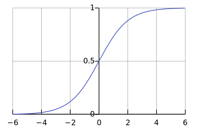
Line 04: This is our "nonlinearity". While it can be several kinds of functions, this nonlinearity maps a function called a "sigmoid". A sigmoid function maps any value to a value between 0 and 1. We use it to convert numbers to probabilities. It also has several other desirable properties for training neural networks.
Line 05:
Notice that this function can also generate the derivative of a sigmoid (when deriv=True). One of the desirable properties of a sigmoid function is that its output can be used to create its derivative. If the sigmoid's output is a variable "out", then the derivative is simply out * (1-out). This is very efficient.
If you're unfamililar with derivatives, just think about it as the slope of the sigmoid function at a given point (as you can see above, different points have different slopes). For more on derivatives, check out this derivatives tutorial from Khan Academy.
Line 10: This initializes our input dataset as a numpy matrix. Each row is a single "training example". Each column corresponds to one of our input nodes. Thus, we have 3 input nodes to the network and 4 training examples.
Line 16: This initializes our output dataset. In this case, I generated the dataset horizontally (with a single row and 4 columns) for space. ".T" is the transpose function. After the transpose, this y matrix has 4 rows with one column. Just like our input, each row is a training example, and each column (only one) is an output node. So, our network has 3 inputs and 1 output.
Line 20: It's good practice to seed your random numbers. Your numbers will still be randomly distributed, but they'll be randomly distributed in exactly the same way each time you train. This makes it easier to see how your changes affect the network.
Line 23:
This is our weight matrix for this neural network. It's called "syn0" to imply "synapse zero". Since we only have 2 layers (input and output), we only need one matrix of weights to connect them. Its dimension is (3,1) because we have 3 inputs and 1 output. Another way of looking at it is that l0 is of size 3 and l1 is of size 1. Thus, we want to connect every node in l0 to every node in l1, which requires a matrix of dimensionality (3,1). :)
Also notice that it is initialized randomly with a mean of zero. There is quite a bit of theory that goes into weight initialization. For now, just take it as a best practice that it's a good idea to have a mean of zero in weight initialization.
Another note is that the "neural network" is really just this matrix. We have "layers" l0 and l1 but they are transient values based on the dataset. We don't save them. All of the learning is stored in the syn0 matrix.
Line 25: This begins our actual network training code. This for loop "iterates" multiple times over the training code to optimize our network to the dataset.
Line 28: Since our first layer, l0, is simply our data. We explicitly describe it as such at this point. Remember that X contains 4 training examples (rows). We're going to process all of them at the same time in this implementation. This is known as "full batch" training. Thus, we have 4 different l0 rows, but you can think of it as a single training example if you want. It makes no difference at this point. (We could load in 1000 or 10,000 if we wanted to without changing any of the code).
Line 29:
This is our prediction step. Basically, we first let the network "try" to predict the output given the input. We will then study how it performs so that we can adjust it to do a bit better for each iteration.
This line contains 2 steps. The first matrix multiplies l0 by syn0. The second passes our output through the sigmoid function. Consider the dimensions of each:
(4 x 3) dot (3 x 1) = (4 x 1)
Matrix multiplication is ordered, such the dimensions in the middle of the equation must be the same. The final matrix generated is thus the number of rows of the first matrix and the number of columns of the second matrix.
Since we loaded in 4 training examples, we ended up with 4 guesses for the correct answer, a (4 x 1) matrix. Each output corresponds with the network's guess for a given input. Perhaps it becomes intuitive why we could have "loaded in" an arbitrary number of training examples. The matrix multiplication would still work out. :)
Line 32: So, given that l1 had a "guess" for each input. We can now compare how well it did by subtracting the true answer (y) from the guess (l1). l1_error is just a vector of positive and negative numbers reflecting how much the network missed.
Line 36: Now we're getting to the good stuff! This is the secret sauce! There's a lot going on in this line, so let's further break it into two parts.
First Part: The Derivative
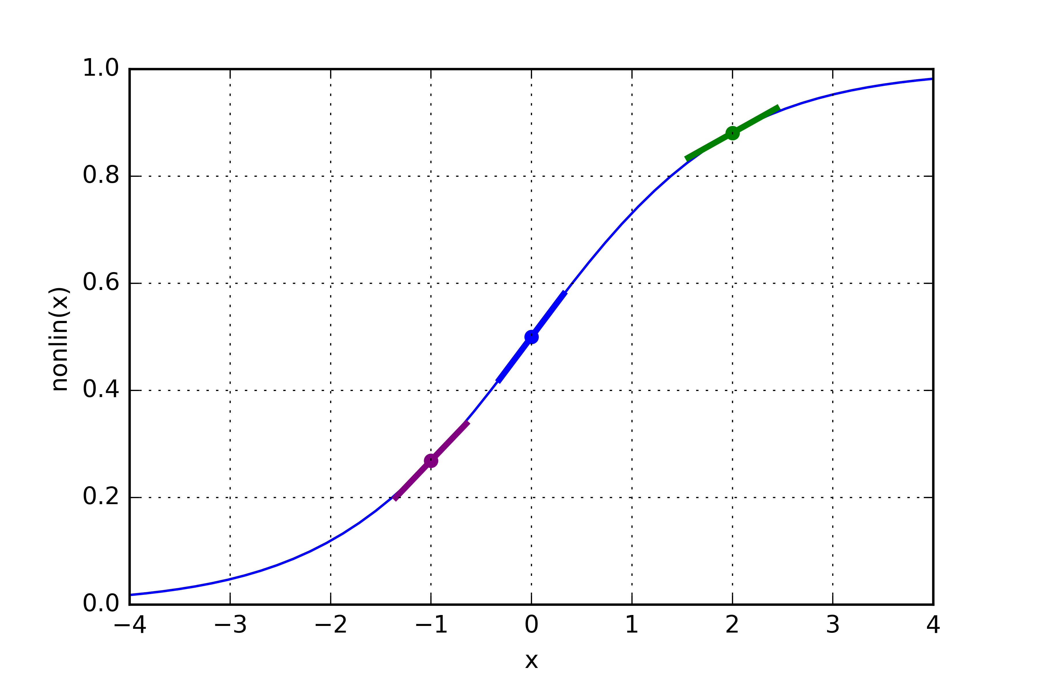
nonlin(l1,True)
If l1 represents these three dots, the code above generates the slopes of the lines below. Notice that very high values such as x=2.0 (green dot) and very low values such as x=-1.0 (purple dot) have rather shallow slopes. The highest slope you can have is at x=0 (blue dot). This plays an important role. Also notice that all derivatives are between 0 and 1.
Entire Statement: The Error Weighted Derivative
l1_delta = l1_error * nonlin(l1,True)
There are more "mathematically precise" ways than "The Error Weighted Derivative" but I think that this captures the intuition. l1_error is a (4,1) matrix. nonlin(l1,True) returns a (4,1) matrix. What we're doing is multiplying them "elementwise". This returns a (4,1) matrix l1_delta with the multiplied values.
When we multiply the "slopes" by the error, we are reducing the error of high confidence predictions. Look at the sigmoid picture again! If the slope was really shallow (close to 0), then the network either had a very high value, or a very low value. This means that the network was quite confident one way or the other. However, if the network guessed something close to (x=0, y=0.5) then it isn't very confident. We update these "wishy-washy" predictions most heavily, and we tend to leave the confident ones alone by multiplying them by a number close to 0.
Line 39:
We are now ready to update our network! Let's take a look at a single training example.
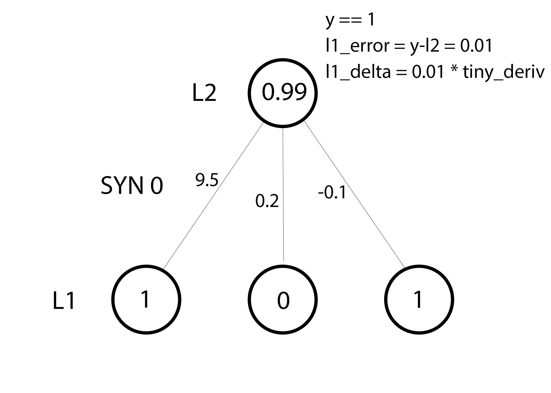 In this training example, we're all setup to update our weights. Let's update the far left weight (9.5).
weight_update = input_value * l1_delta
For the far left weight, this would multiply 1.0 * the l1_delta. Presumably, this would increment 9.5 ever so slightly. Why only a small ammount? Well, the prediction was already very confident, and the prediction was largely correct. A small error and a small slope means a VERY small update. Consider all the weights. It would ever so slightly increase all three.
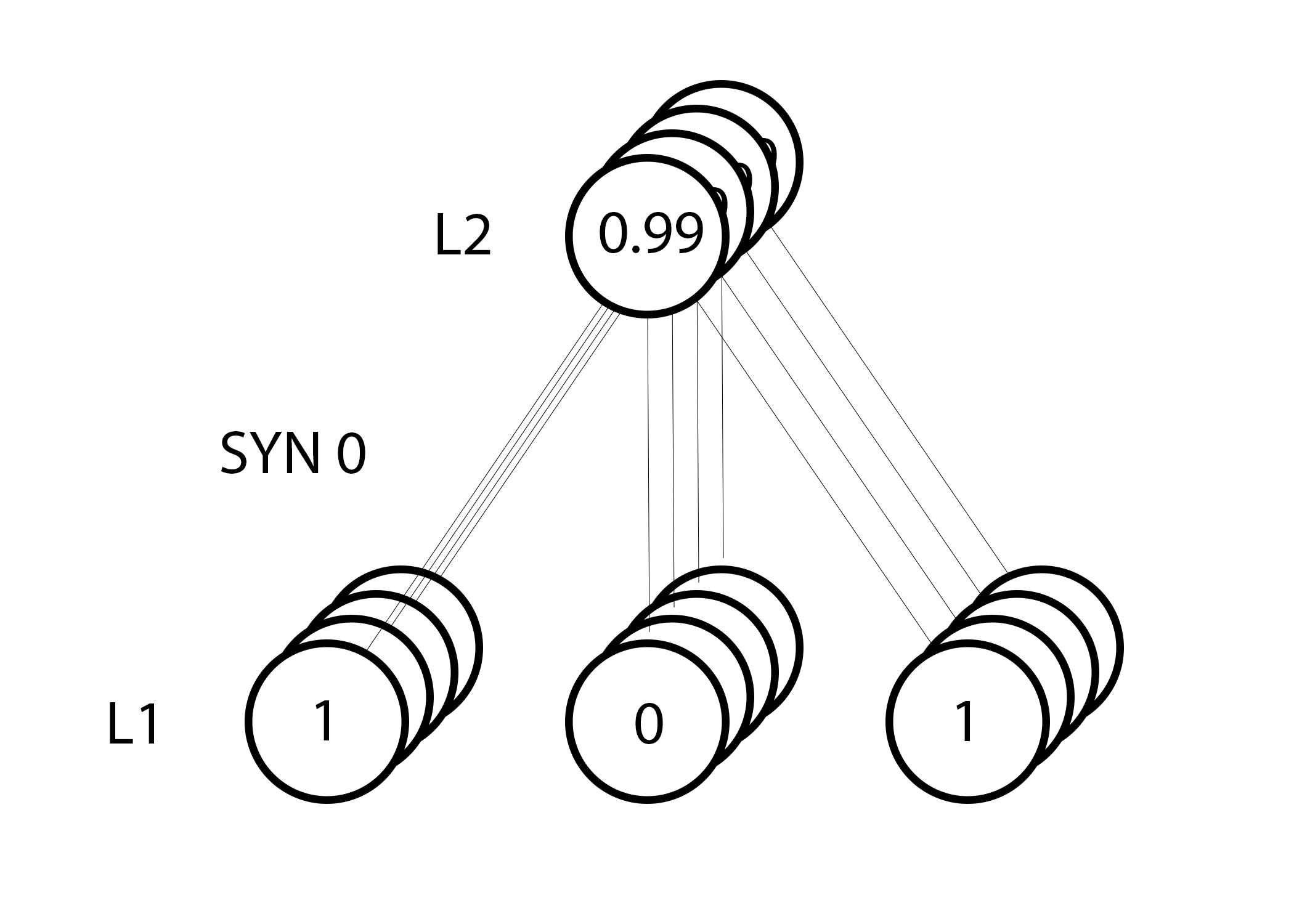
However, because we're using a "full batch" configuration, we're doing the above step on all four training examples. So, it looks a lot more like the image above. So, what does line 39 do? It computes the weight updates for each weight for each training example, sums them, and updates the weights, all in a simple line. Play around with the matrix multiplication and you'll see it do this!
Takeaways:
So, now that we've looked at how the network updates, let's look back at our training data and reflect. When both an input and a output are 1, we increase the weight between them. When an input is 1 and an output is 0, we decrease the weight between them.| Inputs | Output | ||
|---|---|---|---|
| 0 | 0 | 1 | 0 |
| 1 | 1 | 1 | 1 |
| 1 | 0 | 1 | 1 |
| 0 | 1 | 1 | 0 |
Thus, in our four training examples below, the weight from the first input to the output would consistently increment or remain unchanged, whereas the other two weights would find themselves both increasing and decreasing across training examples (cancelling out progress). This phenomenon is what causes our network to learn based on correlations between the input and output.
Part 2: A Slightly Harder Problem
| Inputs | Output | ||
|---|---|---|---|
| 0 | 0 | 1 | 0 |
| 0 | 1 | 1 | 1 |
| 1 | 0 | 1 | 1 |
| 1 | 1 | 1 | 0 |
Consider trying to predict the output column given the two input columns. A key takeway should be that neither columns have any correlation to the output. Each column has a 50% chance of predicting a 1 and a 50% chance of predicting a 0.
So, what's the pattern? It appears to be completely unrelated to column three, which is always 1. However, columns 1 and 2 give more clarity. If either column 1 or 2 are a 1 (but not both!) then the output is a 1. This is our pattern.
This is considered a "nonlinear" pattern because there isn't a direct one-to-one relationship between the input and output. Instead, there is a one-to-one relationship between a combination of inputs, namely columns 1 and 2.

Believe it or not, image recognition is a similar problem. If one had 100 identically sized images of pipes and bicycles, no individual pixel position would directly correlate with the presence of a bicycle or pipe. The pixels might as well be random from a purely statistical point of view. However, certain combinations of pixels are not random, namely the combination that forms the image of a bicycle or a person.
Our Strategy
In order to first combine pixels into something that can then have a one-to-one relationship with the output, we need to add another layer. Our first layer will combine the inputs, and our second layer will then map them to the output using the output of the first layer as input. Before we jump into an implementation though, take a look at this table.
| Inputs (l0) | Hidden Weights (l1) | Output (l2) | |||||
|---|---|---|---|---|---|---|---|
| 0 | 0 | 1 | 0.1 | 0.2 | 0.5 | 0.2 | 0 |
| 0 | 1 | 1 | 0.2 | 0.6 | 0.7 | 0.1 | 1 |
| 1 | 0 | 1 | 0.3 | 0.2 | 0.3 | 0.9 | 1 |
| 1 | 1 | 1 | 0.2 | 0.1 | 0.3 | 0.8 | 0 |
If we randomly initialize our weights, we will get hidden state values for layer 1. Notice anything? The second column (second hidden node), has a slight correlation with the output already! It's not perfect, but it's there. Believe it or not, this is a huge part of how neural networks train. (Arguably, it's the only way that neural networks train.) What the training below is going to do is amplify that correlation. It's both going to update syn1 to map it to the output, and update syn0 to be better at producing it from the input!
Note: The field of adding more layers to model more combinations of relationships such as this is known as "deep learning" because of the increasingly deep layers being modeled.
3 Layer Neural Network:
import numpy as np

def nonlin(x,deriv=False):
	if(deriv==True):
	    return x*(1-x)

	return 1/(1+np.exp(-x))

X = np.array([[0,0,1],
            [0,1,1],
            [1,0,1],
            [1,1,1]])

y = np.array([[0],
			[1],
			[1],
			[0]])

np.random.seed(1)

# randomly initialize our weights with mean 0
syn0 = 2*np.random.random((3,4)) - 1
syn1 = 2*np.random.random((4,1)) - 1

for j in xrange(60000):

	# Feed forward through layers 0, 1, and 2
    l0 = X
    l1 = nonlin(np.dot(l0,syn0))
    l2 = nonlin(np.dot(l1,syn1))

    # how much did we miss the target value?
    l2_error = y - l2

    if (j% 10000) == 0:
        print "Error:" + str(np.mean(np.abs(l2_error)))

    # in what direction is the target value?
    # were we really sure? if so, don't change too much.
    l2_delta = l2_error*nonlin(l2,deriv=True)

    # how much did each l1 value contribute to the l2 error (according to the weights)?
    l1_error = l2_delta.dot(syn1.T)

    # in what direction is the target l1?
    # were we really sure? if so, don't change too much.
    l1_delta = l1_error * nonlin(l1,deriv=True)

    syn1 += l1.T.dot(l2_delta)
    syn0 += l0.T.dot(l1_delta)
Error:0.496410031903
Error:0.00858452565325
Error:0.00578945986251
Error:0.00462917677677
Error:0.00395876528027
Error:0.00351012256786
| Variable | Definition |
|---|---|
| X | Input dataset matrix where each row is a training example |
| y | Output dataset matrix where each row is a training example |
| l0 | First Layer of the Network, specified by the input data |
| l1 | Second Layer of the Network, otherwise known as the hidden layer |
| l2 | Final Layer of the Network, which is our hypothesis, and should approximate the correct answer as we train. |
| syn0 | First layer of weights, Synapse 0, connecting l0 to l1. |
| syn1 | Second layer of weights, Synapse 1 connecting l1 to l2. |
| l2_error | This is the amount that the neural network "missed". |
| l2_delta | This is the error of the network scaled by the confidence. It's almost identical to the error except that very confident errors are muted. |
| l1_error | Weighting l2_delta by the weights in syn1, we can calculate the error in the middle/hidden layer. |
| l1_delta | This is the l1 error of the network scaled by the confidence. Again, it's almost identical to the l1_error except that confident errors are muted. |
Recommendation: open this blog in two screens so you can see the code while you read it. That's kinda what I did while I wrote it. :)
Everything should look very familiar! It's really just 2 of the previous implementation stacked on top of each other. The output of the first layer (l1) is the input to the second layer. The only new thing happening here is on line 43.
Line 43: uses the "confidence weighted error" from l2 to establish an error for l1. To do this, it simply sends the error across the weights from l2 to l1. This gives what you could call a "contribution weighted error" because we learn how much each node value in l1 "contributed" to the error in l2. This step is called "backpropagating" and is the namesake of the algorithm. We then update syn0 using the same steps we did in the 2 layer implementation.
Part 3: Conclusion and Future Work
My Recommendation:
If you're serious about neural networks, I have one recommendation. Try to rebuild this network from memory. I know that might sound a bit crazy, but it seriously helps. If you want to be able to create arbitrary architectures based on new academic papers or read and understand sample code for these different architectures, I think that it's a killer exercise. I think it's useful even if you're using frameworks like Torch, Caffe, or Theano. I worked with neural networks for a couple years before performing this exercise, and it was the best investment of time I've made in the field (and it didn't take long).Future Work
This toy example still needs quite a few bells and whistles to really approach the state-of-the-art architectures. Here's a few things you can look into if you want to further improve your network. (Perhaps I will in a followup post.)
• Alpha
• Bias Units
• Mini-Batches
• Delta Trimming
• Parameterized Layer Sizes
• Regularization
• Dropout
• Momentum
• Batch Normalization
• GPU Compatability
• Other Awesomeness You Implement
Want to Work in Machine Learning?
One of the best things you can do to learn Machine Learning is to have a job where you're practicing Machine Learning professionally. I'd encourage you to check out the positions at Digital Reasoning in your job hunt. If you have questions about any of the positions or about life at Digital Reasoning, feel free to send me a message on my LinkedIn. I'm happy to hear about where you want to go in life, and help you evaluate whether Digital Reasoning could be a good fit.
If none of the positions above feel like a good fit. Continue your search! Machine Learning expertise is one of the most valuable skills in the job market today, and there are many firms looking for practitioners. Perhaps some of these services below will help you in your hunt.
View More Job Search Results