Summary: I learn best with toy code that I can play with. This tutorial teaches gradient descent via a very simple toy example, a short python implementation.
Followup Post: I intend to write a followup post to this one adding popular features leveraged by state-of-the-art approaches (likely Dropout, DropConnect, and Momentum). I'll tweet it out when it's complete @iamtrask. Feel free to follow if you'd be interested in reading more and thanks for all the feedback!
Just Give Me The Code:
import numpy as np
X = np.array([ [0,0,1],[0,1,1],[1,0,1],[1,1,1] ])
y = np.array([[0,1,1,0]]).T
alpha,hidden_dim = (0.5,4)
synapse_0 = 2*np.random.random((3,hidden_dim)) - 1
synapse_1 = 2*np.random.random((hidden_dim,1)) - 1
for j in xrange(60000):
    layer_1 = 1/(1+np.exp(-(np.dot(X,synapse_0))))
    layer_2 = 1/(1+np.exp(-(np.dot(layer_1,synapse_1))))
    layer_2_delta = (layer_2 - y)*(layer_2*(1-layer_2))
    layer_1_delta = layer_2_delta.dot(synapse_1.T) * (layer_1 * (1-layer_1))
    synapse_1 -= (alpha * layer_1.T.dot(layer_2_delta))
    synapse_0 -= (alpha * X.T.dot(layer_1_delta))
Part 1: Optimization
In Part 1, I laid out the basis for backpropagation in a simple neural network. Backpropagation allowed us to measure how each weight in the network contributed to the overall error. This ultimately allowed us to change these weights using a different algorithm, Gradient Descent.
The takeaway here is that backpropagation doesn't optimize! It moves the error information from the end of the network to all the weights inside the network so that a different algorithm can optimize those weights to fit our data. We actually have a plethora of different nonlinear optimization methods that we could use with backpropagation:
A Few Optimization Methods:
• Annealing
• Stochastic Gradient Descent
• AW-SGD (new!)
• Momentum (SGD)
• Nesterov Momentum (SGD)
• AdaGrad
• AdaDelta
• ADAM
• BFGS
• LBFGS
Visualizing the Difference:
• ConvNet.js
• RobertsDionne
Many of these optimizations are good for different purposes, and in some cases several can be used together. In this tutorial, we will walk through Gradient Descent, which is arguably the simplest and most widely used neural network optimization algorithm. By learning about Gradient Descent, we will then be able to improve our toy neural network through parameterization and tuning, and ultimately make it a lot more powerful.
Part 2: Gradient Descent
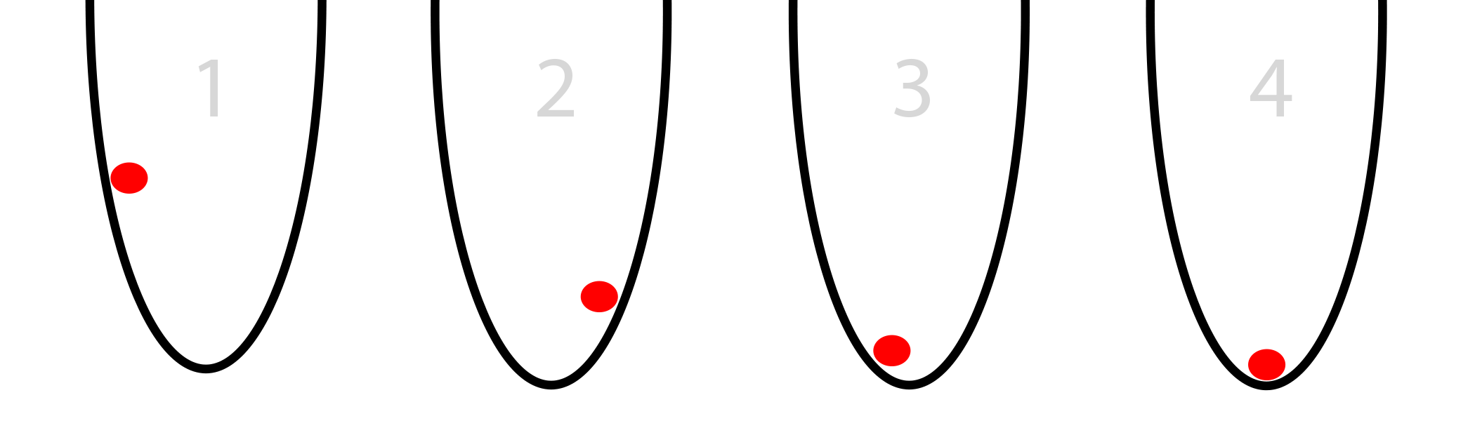
Imagine that you had a red ball inside of a rounded bucket like in the picture below. Imagine further that the red ball is trying to find the bottom of the bucket. This is optimization. In our case, the ball is optimizing it's position (from left to right) to find the lowest point in the bucket.
(pause here.... make sure you got that last sentence.... got it?)
So, to gamify this a bit. The ball has two options, left or right. It has one goal, get as low as possible. So, it needs to press the left and right buttons correctly to find the lowest spot
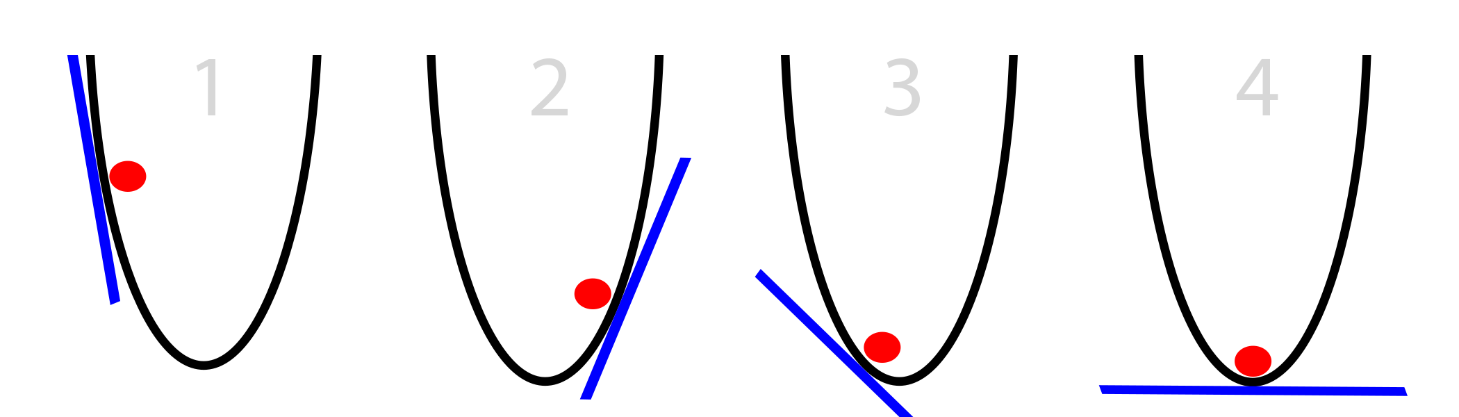
So, what information does the ball use to adjust its position to find the lowest point? The only information it has is the slope of the side of the bucket at its current position, pictured below with the blue line. Notice that when the slope is negative (downward from left to right), the ball should move to the right. However, when the slope is positive, the ball should move to the left. As you can see, this is more than enough information to find the bottom of the bucket in a few iterations. This is a sub-field of optimization called gradient optimization. (Gradient is just a fancy word for slope or steepness).
Oversimplified Gradient Descent:
- Calculate slope at current position
- If slope is negative, move right
- If slope is positive, move left
- (Repeat until slope == 0)
The question is, however, how much should the ball move at each time step? Look at the bucket again. The steeper the slope, the farther the ball is from the bottom. That's helpful! Let's improve our algorithm to leverage this new information. Also, let's assume that the bucket is on an (x,y) plane. So, its location is x (along the bottom). Increasing the ball's "x" position moves it to the right. Decreasing the ball's "x" position moves it to the left.
Naive Gradient Descent:
- Calculate "slope" at current "x" position
- Change x by the negative of the slope. (x = x - slope)
- (Repeat until slope == 0)
Make sure you can picture this process in your head before moving on. This is a considerable improvement to our algorithm. For very positive slopes, we move left by a lot. For only slightly positive slopes, we move left by only a little. As it gets closer and closer to the bottom, it takes smaller and smaller steps until the slope equals zero, at which point it stops. This stopping point is called convergence.
Part 3: Sometimes It Breaks
Gradient Descent isn't perfect. Let's take a look at its issues and how people get around them. This will allow us to improve our network to overcome these issues.
Problem 1: When slopes are too big
How big is too big? Remember our step size is based on the steepness of the slope. Sometimes the slope is so steep that we overshoot by a lot. Overshooting by a little is ok, but sometimes we overshoot by so much that we're even farther away than we started! See below.
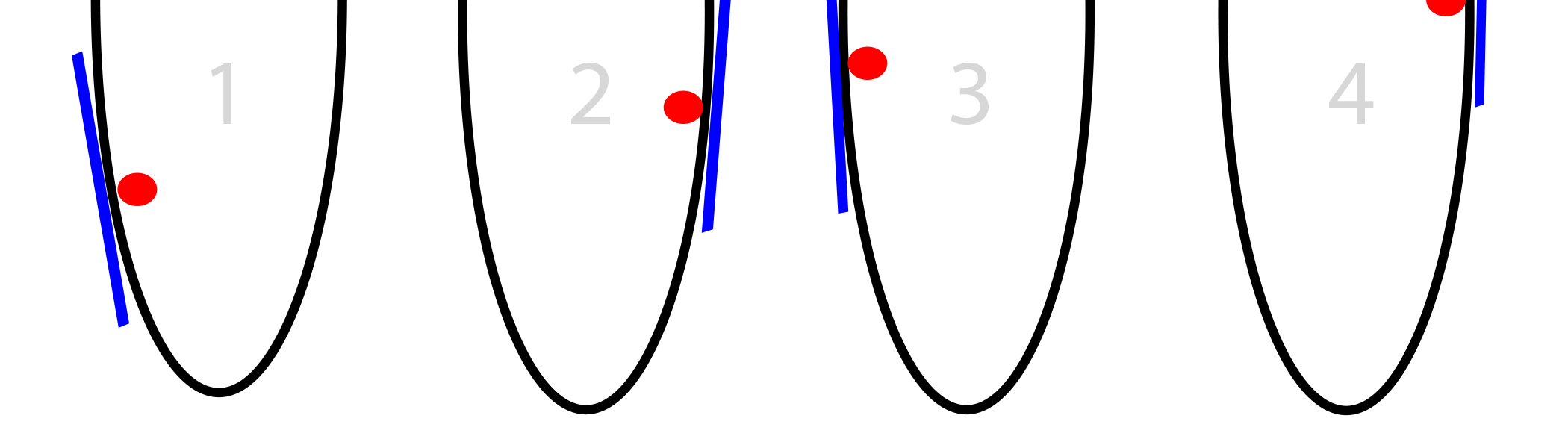
What makes this problem so destructive is that overshooting this far means we land at an EVEN STEEPER slope in the opposite direction. This causes us to overshoot again EVEN FARTHER. This viscious cycle of overshooting leading to more overshooting is called divergence.
Solution 1: Make Slopes Smaller
Lol. This may seem too simple to be true, but it's used in pretty much every neural network. If our gradients are too big, we make them smaller! We do this by multiplying them (all of them) by a single number between 0 and 1 (such as 0.01). This fraction is typically a single float called alpha. When we do this, we don't overshoot and our network converges.
Improved Gradient Descent:
alpha = 0.1 (or some number between 0 and 1)- Calculate "slope" at current "x" position
- x = x - (alpha*slope)
- (Repeat until slope == 0)
Problem 2: Local Minimums
Sometimes your bucket has a funny shape, and following the slope doesn't take you to the absolute lowest point. Consider the picture below.
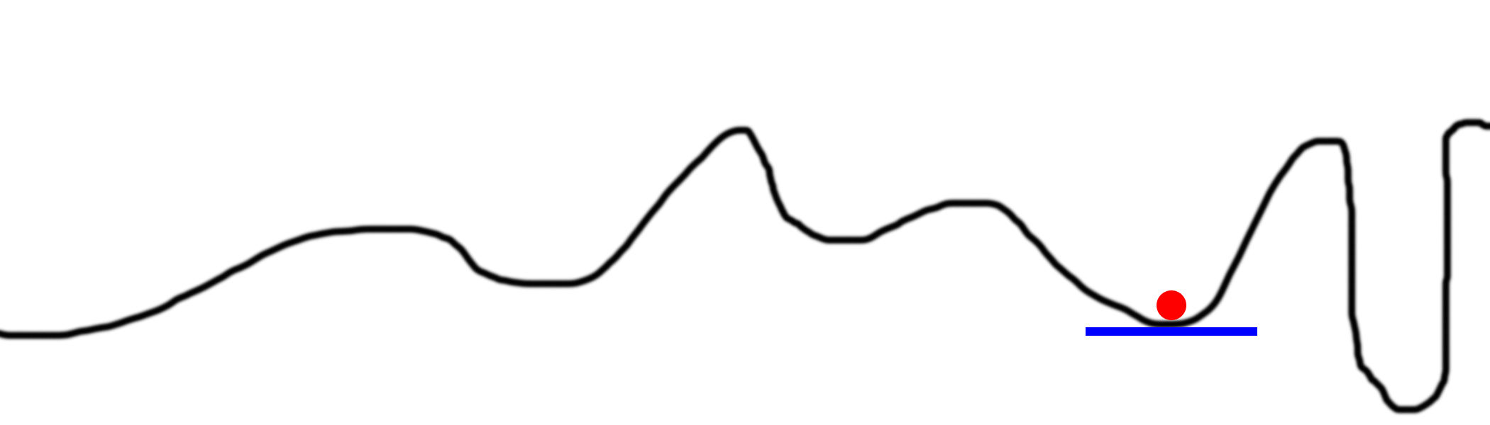
This is by far the most difficult problem with gradient descent. There are a myriad of options to try to overcome this. Generally speaking, they all involve an element of random searching to try lots of different parts of the bucket.
Solution 2: Multiple Random Starting States
There are a myriad of ways in which randomness is used to overcome getting stuck in a local minimum. It begs the question, if we have to use randomness to find the global minimum, why are we still optimizing in the first place? Why not just try randomly? The answer lies in the graph below.
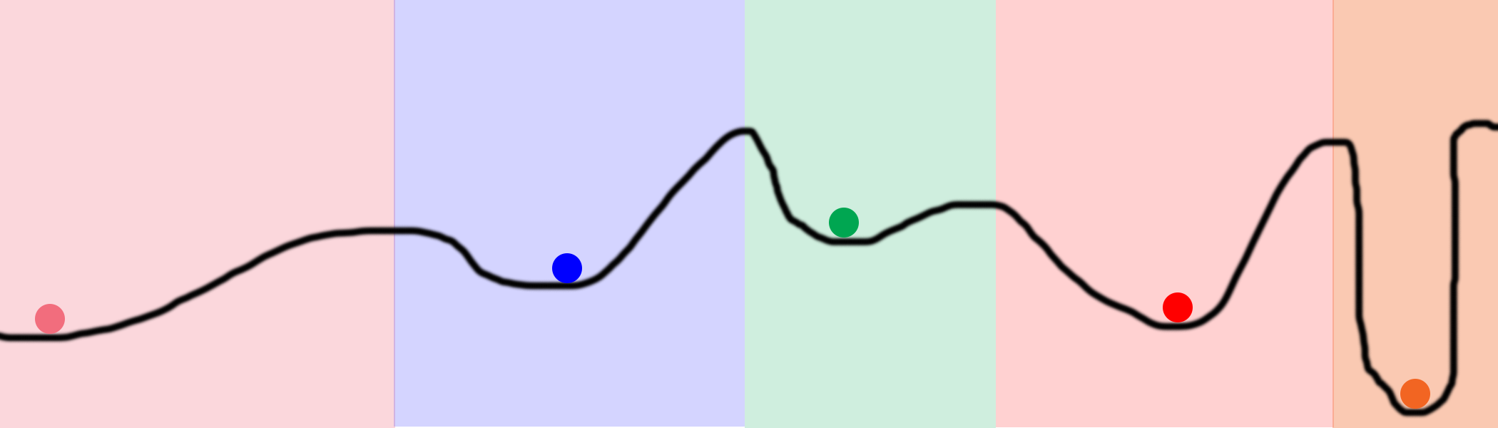
Imagine that we randomly placed 100 balls on this line and started optimizing all of them. If we did so, they would all end up in only 5 positions, mapped out by the five colored balls above. The colored regions represent the domain of each local minimum. For example, if a ball randomly falls within the blue domain, it will converge to the blue minimum. This means that to search the entire space, we only have to randomly find 5 spaces! This is far better than pure random searching, which has to randomly try EVERY space (which could easily be millions of places on this black line depending on the granularity).
In Neural Networks: One way that neural networks accomplish this is by having very large hidden layers. You see, each hidden node in a layer starts out in a different random starting state. This allows each hidden node to converge to different patterns in the network. Parameterizing this size allows the neural network user to potentially try thousands (or tens of billions) of different local minima in a single neural network.
Sidenote 1: This is why neural networks are so powerful! They have the ability to search far more of the space than they actually compute! We can search the entire black line above with (in theory) only 5 balls and a handful of iterations. Searching that same space in a brute force fashion could easily take orders of magnitude more computation.
Sidenote 2: A close eye might ask, "Well, why would we allow a lot of nodes to converge to the same spot? That's actually wasting computational power!" That's an excellent point. The current state-of-the-art approaches to avoiding hidden nodes coming up with the same answer (by searching the same space) are Dropout and Drop-Connect, which I intend to cover in a later post.
Problem 3: When Slopes are Too Small
Neural networks sometimes suffer from the slopes being too small. The answer is also obvious but I wanted to mention it here to expand on its symptoms. Consider the following graph.
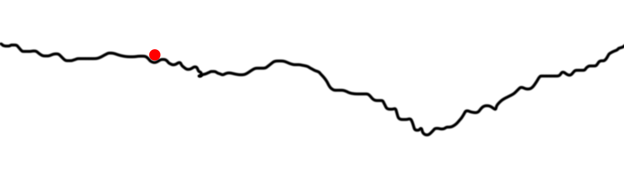
Our little red ball up there is just stuck! If your alpha is too small, this can happen. The ball just drops right into an instant local minimum and ignores the big picture. It doesn't have the umph to get out of the rut.
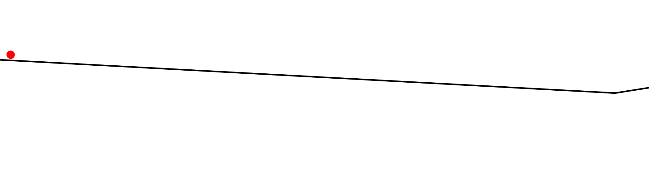
And perhaps the more obvious symptom of deltas that are too small is that the convergence will just take a very, very long time.
Solution 3: Increase the Alpha
As you might expect, the solution to both of these symptoms is to increase the alpha. We might even multiply our deltas by a weight higher than 1. This is very rare, but it does sometimes happen.
Part 4: SGD in Neural Networks
So at this point you might be wondering, how does this relate to neural networks and backpropagation? This is the hardest part, so get ready to hold on tight and take things slow. It's also quite important.
That big nasty curve? In a neural network, we're trying to minimize the error with respect to the weights. So, what that curve represents is the network's error relative to the position of a single weight. So, if we computed the network's error for every possible value of a single weight, it would generate the curve you see above. We would then pick the value of the single weight that has the lowest error (the lowest part of the curve). I say single weight because it's a two-dimensional plot. Thus, the x dimension is the value of the weight and the y dimension is the neural network's error when the weight is at that position.
Let's take a look at what this process looks like in a simple 2 layer neural network.
2 Layer Neural Network:
import numpy as np

# compute sigmoid nonlinearity
def sigmoid(x):
    output = 1/(1+np.exp(-x))
    return output

# convert output of sigmoid function to its derivative
def sigmoid_output_to_derivative(output):
    return output*(1-output)

# input dataset
X = np.array([  [0,1],
                [0,1],
                [1,0],
                [1,0] ])

# output dataset
y = np.array([[0,0,1,1]]).T

# seed random numbers to make calculation
# deterministic (just a good practice)
np.random.seed(1)

# initialize weights randomly with mean 0
synapse_0 = 2*np.random.random((2,1)) - 1

for iter in xrange(10000):

    # forward propagation
    layer_0 = X
    layer_1 = sigmoid(np.dot(layer_0,synapse_0))

    # how much did we miss?
    layer_1_error = layer_1 - y

    # multiply how much we missed by the
    # slope of the sigmoid at the values in l1
    layer_1_delta = layer_1_error * sigmoid_output_to_derivative(layer_1)
    synapse_0_derivative = np.dot(layer_0.T,layer_1_delta)

    # update weights
    synapse_0 -= synapse_0_derivative

print "Output After Training:"
print layer_1
So, in this case, we have a single error at the output (single value), which is computed on line 35. Since we have 2 weights, the output "error plane" is a 3 dimensional space. We can think of this as an (x,y,z) plane, where vertical is the error, and x and y are the values of our two weights in syn0.
Let's try to plot what the error plane looks like for the network/dataset above. So, how do we compute the error for a given set of weights? Lines 31,32,and 35 show us that. If we take that logic and plot the overall error (a single scalar representing the network error over the entire dataset) for every possible set of weights (from -10 to 10 for x and y), it looks something like this.
Don't be intimidated by this. It really is as simple as computing every possible set of weights, and the error that the network generates at each set. x is the first synapse_0 weight and y is the second synapse_0 weight. z is the overall error. As you can see, our output data is positively correlated with the first input data. Thus, the error is minimized when x (the first synapse_0 weight) is high. What about the second synapse_0 weight? How is it optimal?
How Our 2 Layer Neural Network Optimizes
So, given that lines 31,32,and 35 end up computing the error. It can be natural to see that lines 39, 40, and 43 optimize to reduce the error. This is where Gradient Descent is happening! Remember our pseudocode?
Naive Gradient Descent:
- Lines 39 and 40: Calculate "slope" at current "x" position
- Line 43: Change x by the negative of the slope. (x = x - slope)
- Line 28: (Repeat until slope == 0)
It's exactly the same thing! The only thing that has changed is that we have 2 weights that we're optimizing instead of just 1. The logic, however, is identical.
Part 5: Improving our Neural Network
Remember that Gradient Descent had some weaknesses. Now that we have seen how our neural network leverages Gradient Descent, we can improve our network to overcome these weaknesses in the same way that we improved Gradient Descent in Part 3 (the 3 problems and solutions).
Improvement 1: Adding and Tuning the Alpha Parameter
What is Alpha? As described above, the alpha parameter reduces the size of each iteration's update in the simplest way possible. At the very last minute, right before we update the weights, we multiply the weight update by alpha (usually between 0 and 1, thus reducing the size of the weight update). This tiny change to the code has absolutely massive impact on its ability to train.
We're going to jump back to our 3 layer neural network from the first post and add in an alpha parameter at the appropriate place. Then, we're going to run a series of experiments to align all the intuition we developed around alpha with its behavior in live code.
Improved Gradient Descent:
- Calculate "slope" at current "x" position
- Lines 56 and 57: Change x by the negative of the slope scaled by alpha. (x = x - (alpha*slope) )
- (Repeat until slope == 0)
import numpy as np

alphas = [0.001,0.01,0.1,1,10,100,1000]

# compute sigmoid nonlinearity
def sigmoid(x):
    output = 1/(1+np.exp(-x))
    return output

# convert output of sigmoid function to its derivative
def sigmoid_output_to_derivative(output):
    return output*(1-output)

X = np.array([[0,0,1],
            [0,1,1],
            [1,0,1],
            [1,1,1]])

y = np.array([[0],
			[1],
			[1],
			[0]])

for alpha in alphas:
    print "\nTraining With Alpha:" + str(alpha)
    np.random.seed(1)

    # randomly initialize our weights with mean 0
    synapse_0 = 2*np.random.random((3,4)) - 1
    synapse_1 = 2*np.random.random((4,1)) - 1

    for j in xrange(60000):

        # Feed forward through layers 0, 1, and 2
        layer_0 = X
        layer_1 = sigmoid(np.dot(layer_0,synapse_0))
        layer_2 = sigmoid(np.dot(layer_1,synapse_1))

        # how much did we miss the target value?
        layer_2_error = layer_2 - y

        if (j% 10000) == 0:
            print "Error after "+str(j)+" iterations:" + str(np.mean(np.abs(layer_2_error)))

        # in what direction is the target value?
        # were we really sure? if so, don't change too much.
        layer_2_delta = layer_2_error*sigmoid_output_to_derivative(layer_2)

        # how much did each l1 value contribute to the l2 error (according to the weights)?
        layer_1_error = layer_2_delta.dot(synapse_1.T)

        # in what direction is the target l1?
        # were we really sure? if so, don't change too much.
        layer_1_delta = layer_1_error * sigmoid_output_to_derivative(layer_1)

        synapse_1 -= alpha * (layer_1.T.dot(layer_2_delta))
        synapse_0 -= alpha * (layer_0.T.dot(layer_1_delta))
Training With Alpha:0.001
Error after 0 iterations:0.496410031903
Error after 10000 iterations:0.495164025493
Error after 20000 iterations:0.493596043188
Error after 30000 iterations:0.491606358559
Error after 40000 iterations:0.489100166544
Error after 50000 iterations:0.485977857846

Training With Alpha:0.01
Error after 0 iterations:0.496410031903
Error after 10000 iterations:0.457431074442
Error after 20000 iterations:0.359097202563
Error after 30000 iterations:0.239358137159
Error after 40000 iterations:0.143070659013
Error after 50000 iterations:0.0985964298089

Training With Alpha:0.1
Error after 0 iterations:0.496410031903
Error after 10000 iterations:0.0428880170001
Error after 20000 iterations:0.0240989942285
Error after 30000 iterations:0.0181106521468
Error after 40000 iterations:0.0149876162722
Error after 50000 iterations:0.0130144905381

Training With Alpha:1
Error after 0 iterations:0.496410031903
Error after 10000 iterations:0.00858452565325
Error after 20000 iterations:0.00578945986251
Error after 30000 iterations:0.00462917677677
Error after 40000 iterations:0.00395876528027
Error after 50000 iterations:0.00351012256786

Training With Alpha:10
Error after 0 iterations:0.496410031903
Error after 10000 iterations:0.00312938876301
Error after 20000 iterations:0.00214459557985
Error after 30000 iterations:0.00172397549956
Error after 40000 iterations:0.00147821451229
Error after 50000 iterations:0.00131274062834

Training With Alpha:100
Error after 0 iterations:0.496410031903
Error after 10000 iterations:0.125476983855
Error after 20000 iterations:0.125330333528
Error after 30000 iterations:0.125267728765
Error after 40000 iterations:0.12523107366
Error after 50000 iterations:0.125206352756

Training With Alpha:1000
Error after 0 iterations:0.496410031903
Error after 10000 iterations:0.5
Error after 20000 iterations:0.5
Error after 30000 iterations:0.5
Error after 40000 iterations:0.5
Error after 50000 iterations:0.5
So, what did we observe with the different alpha sizes?
Alpha = 0.001
The network with a crazy small alpha didn't hardly converge! This is because we made the weight updates so small that they hardly changed anything, even after 60,000 iterations! This is textbook Problem 3:When Slopes Are Too Small.
Alpha = 0.01
This alpha made a rather pretty convergence. It was quite smooth over the course of the 60,000 iterations but ultimately didn't converge as far as some of the others. This still is textbook Problem 3:When Slopes Are Too Small.
Alpha = 0.1
This alpha made some of progress very quickly but then slowed down a bit. This is still Problem 3. We need to increase alpha some more.
Alpha = 1
As a clever eye might suspect, this had the exact convergence as if we had no alpha at all! Multiplying our weight updates by 1 doesn't change anything. :)
Alpha = 10
Perhaps you were surprised that an alpha that was greater than 1 achieved the best score after only 10,000 iterations! This tells us that our weight updates were being too conservative with smaller alphas. This means that in the smaller alpha parameters (less than 10), the network's weights were generally headed in the right direction, they just needed to hurry up and get there!
Alpha = 100
Now we can see that taking steps that are too large can be very counterproductive. The network's steps are so large that it can't find a reasonable lowpoint in the error plane. This is textbook Problem 1. The Alpha is too big so it just jumps around on the error plane and never "settles" into a local minimum.
Alpha = 1000
And with an extremely large alpha, we see a textbook example of divergence, with the error increasing instead of decreasing... hardlining at 0.5. This is a more extreme version of Problem 1 where it overcorrectly whildly and ends up very far away from any local minimums.
Let's Take a Closer Look
import numpy as np

alphas = [0.001,0.01,0.1,1,10,100,1000]

# compute sigmoid nonlinearity
def sigmoid(x):
    output = 1/(1+np.exp(-x))
    return output

# convert output of sigmoid function to its derivative
def sigmoid_output_to_derivative(output):
    return output*(1-output)

X = np.array([[0,0,1],
            [0,1,1],
            [1,0,1],
            [1,1,1]])

y = np.array([[0],
			[1],
			[1],
			[0]])


for alpha in alphas:
    print "\nTraining With Alpha:" + str(alpha)
    np.random.seed(1)

    # randomly initialize our weights with mean 0
    synapse_0 = 2*np.random.random((3,4)) - 1
    synapse_1 = 2*np.random.random((4,1)) - 1

    prev_synapse_0_weight_update = np.zeros_like(synapse_0)
    prev_synapse_1_weight_update = np.zeros_like(synapse_1)

    synapse_0_direction_count = np.zeros_like(synapse_0)
    synapse_1_direction_count = np.zeros_like(synapse_1)

    for j in xrange(60000):

        # Feed forward through layers 0, 1, and 2
        layer_0 = X
        layer_1 = sigmoid(np.dot(layer_0,synapse_0))
        layer_2 = sigmoid(np.dot(layer_1,synapse_1))

        # how much did we miss the target value?
        layer_2_error = y - layer_2

        if (j% 10000) == 0:
            print "Error:" + str(np.mean(np.abs(layer_2_error)))

        # in what direction is the target value?
        # were we really sure? if so, don't change too much.
        layer_2_delta = layer_2_error*sigmoid_output_to_derivative(layer_2)

        # how much did each l1 value contribute to the l2 error (according to the weights)?
        layer_1_error = layer_2_delta.dot(synapse_1.T)

        # in what direction is the target l1?
        # were we really sure? if so, don't change too much.
        layer_1_delta = layer_1_error * sigmoid_output_to_derivative(layer_1)

        synapse_1_weight_update = (layer_1.T.dot(layer_2_delta))
        synapse_0_weight_update = (layer_0.T.dot(layer_1_delta))

        if(j > 0):
            synapse_0_direction_count += np.abs(((synapse_0_weight_update > 0)+0) - ((prev_synapse_0_weight_update > 0) + 0))
            synapse_1_direction_count += np.abs(((synapse_1_weight_update > 0)+0) - ((prev_synapse_1_weight_update > 0) + 0))

        synapse_1 += alpha * synapse_1_weight_update
        synapse_0 += alpha * synapse_0_weight_update

        prev_synapse_0_weight_update = synapse_0_weight_update
        prev_synapse_1_weight_update = synapse_1_weight_update

    print "Synapse 0"
    print synapse_0

    print "Synapse 0 Update Direction Changes"
    print synapse_0_direction_count

    print "Synapse 1"
    print synapse_1

    print "Synapse 1 Update Direction Changes"
    print synapse_1_direction_count
Training With Alpha:0.001
Error:0.496410031903
Error:0.495164025493
Error:0.493596043188
Error:0.491606358559
Error:0.489100166544
Error:0.485977857846
Synapse 0
[[-0.28448441  0.32471214 -1.53496167 -0.47594822]
 [-0.7550616  -1.04593014 -1.45446052 -0.32606771]
 [-0.2594825  -0.13487028 -0.29722666  0.40028038]]
Synapse 0 Update Direction Changes
[[ 0.  0.  0.  0.]
 [ 0.  0.  0.  0.]
 [ 1.  0.  1.  1.]]
Synapse 1
[[-0.61957526]
 [ 0.76414675]
 [-1.49797046]
 [ 0.40734574]]
Synapse 1 Update Direction Changes
[[ 1.]
 [ 1.]
 [ 0.]
 [ 1.]]

Training With Alpha:0.01
Error:0.496410031903
Error:0.457431074442
Error:0.359097202563
Error:0.239358137159
Error:0.143070659013
Error:0.0985964298089
Synapse 0
[[ 2.39225985  2.56885428 -5.38289334 -3.29231397]
 [-0.35379718 -4.6509363  -5.67005693 -1.74287864]
 [-0.15431323 -1.17147894  1.97979367  3.44633281]]
Synapse 0 Update Direction Changes
[[ 1.  1.  0.  0.]
 [ 2.  0.  0.  2.]
 [ 4.  2.  1.  1.]]
Synapse 1
[[-3.70045078]
 [ 4.57578637]
 [-7.63362462]
 [ 4.73787613]]
Synapse 1 Update Direction Changes
[[ 2.]
 [ 1.]
 [ 0.]
 [ 1.]]

Training With Alpha:0.1
Error:0.496410031903
Error:0.0428880170001
Error:0.0240989942285
Error:0.0181106521468
Error:0.0149876162722
Error:0.0130144905381
Synapse 0
[[ 3.88035459  3.6391263  -5.99509098 -3.8224267 ]
 [-1.72462557 -5.41496387 -6.30737281 -3.03987763]
 [ 0.45953952 -1.77301389  2.37235987  5.04309824]]
Synapse 0 Update Direction Changes
[[ 1.  1.  0.  0.]
 [ 2.  0.  0.  2.]
 [ 4.  2.  1.  1.]]
Synapse 1
[[-5.72386389]
 [ 6.15041318]
 [-9.40272079]
 [ 6.61461026]]
Synapse 1 Update Direction Changes
[[ 2.]
 [ 1.]
 [ 0.]
 [ 1.]]

Training With Alpha:1
Error:0.496410031903
Error:0.00858452565325
Error:0.00578945986251
Error:0.00462917677677
Error:0.00395876528027
Error:0.00351012256786
Synapse 0
[[ 4.6013571   4.17197193 -6.30956245 -4.19745118]
 [-2.58413484 -5.81447929 -6.60793435 -3.68396123]
 [ 0.97538679 -2.02685775  2.52949751  5.84371739]]
Synapse 0 Update Direction Changes
[[ 1.  1.  0.  0.]
 [ 2.  0.  0.  2.]
 [ 4.  2.  1.  1.]]
Synapse 1
[[ -6.96765763]
 [  7.14101949]
 [-10.31917382]
 [  7.86128405]]
Synapse 1 Update Direction Changes
[[ 2.]
 [ 1.]
 [ 0.]
 [ 1.]]

Training With Alpha:10
Error:0.496410031903
Error:0.00312938876301
Error:0.00214459557985
Error:0.00172397549956
Error:0.00147821451229
Error:0.00131274062834
Synapse 0
[[ 4.52597806  5.77663165 -7.34266481 -5.29379829]
 [ 1.66715206 -7.16447274 -7.99779235 -1.81881849]
 [-4.27032921 -3.35838279  3.44594007  4.88852208]]
Synapse 0 Update Direction Changes
[[  7.  19.   2.   6.]
 [  7.   2.   0.  22.]
 [ 19.  26.   9.  17.]]
Synapse 1
[[ -8.58485788]
 [ 10.1786297 ]
 [-14.87601886]
 [  7.57026121]]
Synapse 1 Update Direction Changes
[[ 22.]
 [ 15.]
 [  4.]
 [ 15.]]

Training With Alpha:100
Error:0.496410031903
Error:0.125476983855
Error:0.125330333528
Error:0.125267728765
Error:0.12523107366
Error:0.125206352756
Synapse 0
[[-17.20515374   1.89881432 -16.95533155  -8.23482697]
 [  5.70240659 -17.23785161  -9.48052574  -7.92972576]
 [ -4.18781704  -0.3388181    2.82024759  -8.40059859]]
Synapse 0 Update Direction Changes
[[  8.   7.   3.   2.]
 [ 13.   8.   2.   4.]
 [ 16.  13.  12.   8.]]
Synapse 1
[[  9.68285369]
 [  9.55731916]
 [-16.0390702 ]
 [  6.27326973]]
Synapse 1 Update Direction Changes
[[ 13.]
 [ 11.]
 [ 12.]
 [ 10.]]

Training With Alpha:1000
Error:0.496410031903
Error:0.5
Error:0.5
Error:0.5
Error:0.5
Error:0.5
Synapse 0
[[-56.06177241  -4.66409623  -5.65196179 -23.05868769]
 [ -4.52271708  -4.78184499 -10.88770202 -15.85879101]
 [-89.56678495  10.81119741  37.02351518 -48.33299795]]
Synapse 0 Update Direction Changes
[[ 3.  2.  4.  1.]
 [ 1.  2.  2.  1.]
 [ 6.  6.  4.  1.]]
Synapse 1
[[  25.16188889]
 [  -8.68235535]
 [-116.60053379]
 [  11.41582458]]
Synapse 1 Update Direction Changes
[[ 7.]
 [ 7.]
 [ 7.]
 [ 3.]]
What I did in the above code was count the number of times a derivative changed direction. That's the "Update Direction Changes" readout at the end of training. If a slope (derivative) changes direction, it means that it passed OVER the local minimum and needs to go back. If it never changes direction, it means that it probably didn't go far enough.
A Few Takeaways:
- When the alpha was tiny, the derivatives almost never changed direction.
- When the alpha was optimal, the derivative changed directions a TON.
- When the alpha was huge, the derivative changed directions a medium amount.
- When the alpha was tiny, the weights ended up being reasonably small too
- When the alpha was huge, the weights got huge too!
Improvement 2: Parameterizing the Size of the Hidden Layer
Being able to increase the size of the hidden layer increases the amount of search space that we converge to in each iteration. Consider the network and output
import numpy as np

alphas = [0.001,0.01,0.1,1,10,100,1000]
hiddenSize = 32

# compute sigmoid nonlinearity
def sigmoid(x):
    output = 1/(1+np.exp(-x))
    return output

# convert output of sigmoid function to its derivative
def sigmoid_output_to_derivative(output):
    return output*(1-output)

X = np.array([[0,0,1],
            [0,1,1],
            [1,0,1],
            [1,1,1]])

y = np.array([[0],
			[1],
			[1],
			[0]])

for alpha in alphas:
    print "\nTraining With Alpha:" + str(alpha)
    np.random.seed(1)

    # randomly initialize our weights with mean 0
    synapse_0 = 2*np.random.random((3,hiddenSize)) - 1
    synapse_1 = 2*np.random.random((hiddenSize,1)) - 1

    for j in xrange(60000):

        # Feed forward through layers 0, 1, and 2
        layer_0 = X
        layer_1 = sigmoid(np.dot(layer_0,synapse_0))
        layer_2 = sigmoid(np.dot(layer_1,synapse_1))

        # how much did we miss the target value?
        layer_2_error = layer_2 - y

        if (j% 10000) == 0:
            print "Error after "+str(j)+" iterations:" + str(np.mean(np.abs(layer_2_error)))

        # in what direction is the target value?
        # were we really sure? if so, don't change too much.
        layer_2_delta = layer_2_error*sigmoid_output_to_derivative(layer_2)

        # how much did each l1 value contribute to the l2 error (according to the weights)?
        layer_1_error = layer_2_delta.dot(synapse_1.T)

        # in what direction is the target l1?
        # were we really sure? if so, don't change too much.
        layer_1_delta = layer_1_error * sigmoid_output_to_derivative(layer_1)

        synapse_1 -= alpha * (layer_1.T.dot(layer_2_delta))
        synapse_0 -= alpha * (layer_0.T.dot(layer_1_delta))
Training With Alpha:0.001
Error after 0 iterations:0.496439922501
Error after 10000 iterations:0.491049468129
Error after 20000 iterations:0.484976307027
Error after 30000 iterations:0.477830678793
Error after 40000 iterations:0.46903846539
Error after 50000 iterations:0.458029258565

Training With Alpha:0.01
Error after 0 iterations:0.496439922501
Error after 10000 iterations:0.356379061648
Error after 20000 iterations:0.146939845465
Error after 30000 iterations:0.0880156127416
Error after 40000 iterations:0.065147819275
Error after 50000 iterations:0.0529658087026

Training With Alpha:0.1
Error after 0 iterations:0.496439922501
Error after 10000 iterations:0.0305404908386
Error after 20000 iterations:0.0190638725334
Error after 30000 iterations:0.0147643907296
Error after 40000 iterations:0.0123892429905
Error after 50000 iterations:0.0108421669738

Training With Alpha:1
Error after 0 iterations:0.496439922501
Error after 10000 iterations:0.00736052234249
Error after 20000 iterations:0.00497251705039
Error after 30000 iterations:0.00396863978159
Error after 40000 iterations:0.00338641021983
Error after 50000 iterations:0.00299625684932

Training With Alpha:10
Error after 0 iterations:0.496439922501
Error after 10000 iterations:0.00224922117381
Error after 20000 iterations:0.00153852153014
Error after 30000 iterations:0.00123717718456
Error after 40000 iterations:0.00106119569132
Error after 50000 iterations:0.000942641990774

Training With Alpha:100
Error after 0 iterations:0.496439922501
Error after 10000 iterations:0.5
Error after 20000 iterations:0.5
Error after 30000 iterations:0.5
Error after 40000 iterations:0.5
Error after 50000 iterations:0.5

Training With Alpha:1000
Error after 0 iterations:0.496439922501
Error after 10000 iterations:0.5
Error after 20000 iterations:0.5
Error after 30000 iterations:0.5
Error after 40000 iterations:0.5
Error after 50000 iterations:0.5
Notice that the best error with 32 nodes is 0.0009 whereas the best error with 4 hidden nodes was only 0.0013. This might not seem like much, but it's an important lesson. We do not need any more than 3 nodes to represent this dataset. However, because we had more nodes when we started, we searched more of the space in each iteration and ultimately converged faster. Even though this is very marginal in this toy problem, this affect plays a huge role when modeling very complex datasets.
Part 6: Conclusion and Future Work
My Recommendation:
If you're serious about neural networks, I have one recommendation. Try to rebuild this network from memory. I know that might sound a bit crazy, but it seriously helps. If you want to be able to create arbitrary architectures based on new academic papers or read and understand sample code for these different architectures, I think that it's a killer exercise. I think it's useful even if you're using frameworks like Torch, Caffe, or Theano. I worked with neural networks for a couple years before performing this exercise, and it was the best investment of time I've made in the field (and it didn't take long).Future Work
This toy example still needs quite a few bells and whistles to really approach the state-of-the-art architectures. Here's a few things you can look into if you want to further improve your network. (Perhaps I will in a followup post.)
• Bias Units
• Mini-Batches
• Delta Trimming
• Parameterized Layer Sizes
• Regularization
• Dropout
• Momentum
• Batch Normalization
• GPU Compatability
• Other Awesomeness You Implement
Want to Work in Machine Learning?
One of the best things you can do to learn Machine Learning is to have a job where you're practicing Machine Learning professionally. I'd encourage you to check out the positions at Digital Reasoning in your job hunt. If you have questions about any of the positions or about life at Digital Reasoning, feel free to send me a message on my LinkedIn. I'm happy to hear about where you want to go in life, and help you evaluate whether Digital Reasoning could be a good fit.
If none of the positions above feel like a good fit. Continue your search! Machine Learning expertise is one of the most valuable skills in the job market today, and there are many firms looking for practitioners. Perhaps some of these services below will help you in your hunt.
View More Job Search Results