TLDR: In this blogpost, we're going to prototype (from scratch) and learn the intuitions behind DeepMind's recently proposed Decoupled Neural Interfaces Using Synthetic Gradients paper.
I typically tweet out new blogposts when they're complete at @iamtrask. Feel free to follow if you'd be interested in reading more in the future and thanks for all the feedback!
Part 1: Synthetic Gradients Overview
Normally, a neural network compares its predictions to a dataset to decide how to update its weights. It then uses backpropagation to figure out how each weight should move in order to make the prediction more accurate. However, with Synthetic Gradients, individual layers instead make a "best guess" for what they think the data will say, and then update their weights according to this guess. This "best guess" is called a Synthetic Gradient. The data is only used to help update each layer's "guesser" or Synthetic Gradient generator. This allows for (most of the time), individual layers to learn in isolation, which increases the speed of training.
Edit: This paper also adds great intuitions on how/why Synthetic Gradients are so effective
 Source: Decoupled Neural Interfaces Using Synthetic Gradients
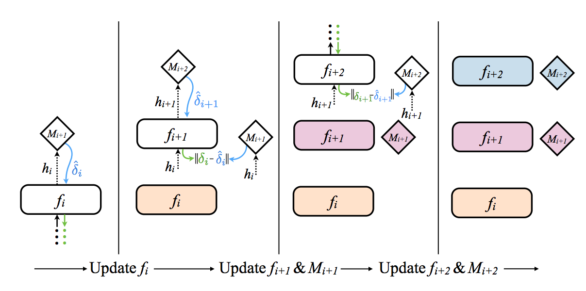
The graphic above (from the paper) gives a very intuitive picture for what’s going on (from left to right). The squares with rounded off corners are layers and the diamond shaped objects are (what I call) the Synthetic Gradient generators. Let’s start with how a regular neural network layer is updated.
Part 2: Using Synthetic Gradients
Let's start by ignoring how the Synthetic Gradients are created and instead just look at how the are used. The far left box shows how these can work to update the first layer in a neural network. The first layer forward propagates into the Synthetic Gradient generator (M i+1), which then returns a gradient. This gradient is used instead of the real gradient (which would take a full forward propagation and backpropagation to compute). The weights are then updated as normal, pretending that this Synthetic Gradient is the real gradient. If you need a refresher on how weights are updated with gradients, check out A Neural Network in 11 Lines of Python and perhaps the followup post on Gradient Descent.
So, in short, Synthetic Gradients are used just like normal gradients, and for some magical reason they seem to be accurate (without consulting the data)! Seems like magic? Let’s see how they’re made.
Part 3: Generating Synthetic Gradients
Ok, this part is really clever, and frankly it's amazing that it works. How do you generate Synthetic Gradients for a neural network? Well, you use another network of course! Synthetic Gradient genenerators are nothing other than a neural network that is trained to take the output of a layer and predict the gradient that will likely happen at that layer.
A Sidenote: Related Work by Geoffrey Hinton
This actually reminds me of some work that Geoffrey Hinton did a couple years ago in which he showed that random feedback weights support learning in deep neural networks. Basically, you can backpropagate through randomly generated matrices and still accomplish learning. Furthermore, he showed that it had a kind of regularization affect. It was some interesting work for sure.
Ok, back to Synthetic Gradients. So, now we know that Synthetic Gradients are trained by another neural network that learns to predict the gradient at a step given the output at that step. The paper also says that any other relevant information could be used as input to the Synthetic Gradient generator network, but in the paper it seems like just the output of the layer is used for normal feedforwards networks. Furthermore, the paper even states that a single linear layer can be used as the Synthetic Gradient generator. Amazing. We're going to try that out.
How do we learn the network that generates Synthetic Gradients?
This begs the question, how do we learn the neural networks that generate our Synthetic Gradients? Well, as it turns out, when we perform full forward and backpropagation, we actually get the "correct" gradient. We can compare this to our "synthetic" gradient in the same way we normally compare the output of a neural network to the dataset. Thus, we can train our Synthetic Gradient networks by pretending that our "true gradients" are coming from mythical dataset... so we train them like normal. Neat!
Wait... if our Synthetic Gradient Network requires backprop... what's the point?
Excellent question! The whole point of this technique was to allow individual neural networks to train without waiting on each other to finish forward and backpropagating. If our Synthetic Gradient networks require waiting for a full forward/backprop step, then we're back where we started but with more computation going on (even worse!). For the answer, let's revisit this visualization from the paper.
Source: Decoupled Neural Interfaces Using Synthetic Gradients
Focus on the second section from the left. See how the gradient (M i+2) backpropagates through (f i+1) and into M(i+1)? As you can see, each synthetic gradient generator is actually only trained using the Synthetic Gradients generated from the next layer. Thus, only the last layer actually trains on the data. All the other layers, including the Synthetic Gradient generator networks, train based on Synthetic Gradients. Thus, the network can train with each layer only having to wait on the synthetic gradient from the following layer (which has no other dependencies). Very cool!
Part 4: A Baseline Neural Network
Time to start coding! To get things started (so we have an easier frame of reference), I'm going to start with a vanilla neural network trained with backpropagation, styled in the same way as A Neural Network in 11 Lines of Python. (So, if it doesn't make sense, just go read that post and come back). However, I'm going to add an additional layer, but that shoudln't be a problem for comprehension. I just figured that since we're all about reducing dependencies, having more layers might make for a better illustration.
As far as the dataset we're training on, I'm going to genereate a synthetic dataset (har! har!) using binary addition. So, the network will take two, random binary numbers and predict their sum (also a binary number). The nice thing is that this gives us the flexibility to increase the dimensionality (~difficulty) of the task as needed. Here's the code for generating the dataset.
And here's the code for a vanilla neural network training on that dataset.
Now, at this point I really feel its necessary to do something that I almost never do in the context of learning, add a bit of object oriented structure. Normally, this obfuscates the network a little bit and makes it harder to see (from a high level) what's going on (relative to just reading a python script). However, since this post is about "Decoupled Neural Interfaces" and the benefits that they offer, it's really pretty hard to explain things without actually having those interfaces be reasonably decoupled.So, to make learning a little bit easier, I'm first going to convert the network above into exactly the same network but with a "Layer" class object that we'll soon convert into a DNI. Let's take a look at this Layer object.
class Layer(object):

    def __init__(self,input_dim, output_dim,nonlin,nonlin_deriv):

        self.weights = (np.random.randn(input_dim, output_dim) * 0.2) - 0.1
        self.nonlin = nonlin
        self.nonlin_deriv = nonlin_deriv

    def forward(self,input):
        self.input = input
        self.output = self.nonlin(self.input.dot(self.weights))
        return self.output

    def backward(self,output_delta):
        self.weight_output_delta = output_delta * self.nonlin_deriv(self.output)
        return self.weight_output_delta.dot(self.weights.T)

    def update(self,alpha=0.1):
        self.weights -= self.input.T.dot(self.weight_output_delta) * alpha
In this Layer class, we have several class variables. weights is the matrix we use for a linear transformation from input to output (just like a normal linear layer). Optionally, we can also include an output nonlin function which will put a non-linearity on the output of our network. If we don't want a non-linearity, we can simply set this value to lambda x:x. In our case, we're going to pass in the "sigmoid" function.
The second function we pass in is nonlin_deriv which is a special derivative function. This function needs to take the output from our nonlinearity and convert it to the derivative. For sigmoid, this is simply (out * (1 - out)) where "out" is the output of the sigmoid. This particular function exists for pretty much all of the common neural network nonlinearities.
Now, let's take a look at the various methods in this class. forward does what it's name implies. It forward propagates through the layer, first through a linear transformation, and then through the nonlin function. backward accepts a output_delta paramter, which represents the real gradient (as opposed to a synthetic one) coming back from the next layer during backpropagation. We then use this to compute self.weight_output_delta, which is the derivative at the output of our weights (just inside the nonlinearity). Finally, it backpropagates the error to send to the previous layer and returns it.
update is perhaps the simplest method of all. It simply takes the derivative at the output of the weights and uses it to perform a weight update. If any of these steps don't make sense to you, again, consult A Neural Network in 11 Lines of Python and come back. If everything makes sense, then let's see our layer objects in the context of training.
layer_1 = Layer(input_dim,layer_1_dim,sigmoid,sigmoid_out2deriv)
layer_2 = Layer(layer_1_dim,layer_2_dim,sigmoid,sigmoid_out2deriv)
layer_3 = Layer(layer_2_dim, output_dim,sigmoid, sigmoid_out2deriv)

for iter in range(iterations):
    error = 0

    for batch_i in range(int(len(x) / batch_size)):
        batch_x = x[(batch_i * batch_size):(batch_i+1)*batch_size]
        batch_y = y[(batch_i * batch_size):(batch_i+1)*batch_size]

        layer_1_out = layer_1.forward(batch_x)
        layer_2_out = layer_2.forward(layer_1_out)
        layer_3_out = layer_3.forward(layer_2_out)

        layer_3_delta = layer_3_out - batch_y
        layer_2_delta = layer_3.backward(layer_3_delta)
        layer_1_delta = layer_2.backward(layer_2_delta)
        layer_1.backward(layer_1_delta)

        layer_1.update()
        layer_2.update()
        layer_3.update()
Given a dataset x and y, this is how we use our new layer objects. If you compare it to the script from before, pretty much everything happens in pretty much the same places. I just swapped out the script versions of the neural network for the method calls
So, all we've really done is taken the steps in the script from the previous neural network and split them into distinct functions inside of a class. Below, we can see this layer in action.
If you pull both the previous network and this network into Jupyter notebooks, you'll see that the random seeds cause these networks to have exactly the same values. It seems that Trinket.io might not have perfect random seeding, such that these networks reach nearly identical values. However, I assure you that the networks are identical. If this network doesn't make sense to you, don't move on. Be sure you're comfortable with how this abstraction works before moving forward, as it's going to get a bit more complex below.
Part 6: Synthetic Gradients Based on Layer Output
Ok, so now we're going to use a very similar interface to the onee to integrate what we learned about Synthetic Gradients into our Layer object (and rename it DNI). First, I'm going to show you the class, and then I'll explain it. Check it out!
class DNI(object):

    def __init__(self,input_dim, output_dim,nonlin,nonlin_deriv,alpha = 0.1):

        # same as before
        self.weights = (np.random.randn(input_dim, output_dim) * 0.2) - 0.1
        self.nonlin = nonlin
        self.nonlin_deriv = nonlin_deriv


        # new stuff
        self.weights_synthetic_grads = (np.random.randn(output_dim,output_dim) * 0.2) - 0.1
        self.alpha = alpha

    # used to be just "forward", but now we update during the forward pass using Synthetic Gradients :)
    def forward_and_synthetic_update(self,input):

    	# cache input
        self.input = input

        # forward propagate
        self.output = self.nonlin(self.input.dot(self.weights))

        # generate synthetic gradient via simple linear transformation
        self.synthetic_gradient = self.output.dot(self.weights_synthetic_grads)

        # update our regular weights using synthetic gradient
        self.weight_synthetic_gradient = self.synthetic_gradient * self.nonlin_deriv(self.output)
        self.weights += self.input.T.dot(self.weight_synthetic_gradient) * self.alpha

        # return backpropagated synthetic gradient (this is like the output of "backprop" method from the Layer class)
        # also return forward propagated output (feels weird i know... )
        return self.weight_synthetic_gradient.dot(self.weights.T), self.output

    # this is just like the "update" method from before... except it operates on the synthetic weights
    def update_synthetic_weights(self,true_gradient):
        self.synthetic_gradient_delta = self.synthetic_gradient - true_gradient
        self.weights_synthetic_grads += self.output.T.dot(self.synthetic_gradient_delta) * self.alpha
So, the first big change. We have some new class variables. The only one that really matters is the self.weights_synthetic_grads variable, which is our Synthetic Generator neural network (just a linear layer... i.e., ...just a matrix).
Forward And Synthetic Update:The forward method has changed to forward_and_synthetic_update. Remember how we don't need any other part of the network to make our weight update? This is where the magic happens. First, forward propagation occurs like normal (line 22). Then, we generate our synthetic gradient by passing our output through a non-linearity. This part could be a more complicated neural network, but we've instead decided to keep things simple and just use a simple linear layer to generate our synthetic gradients. After we've got our gradient, we go ahead and update our normal weights (lines 28 and 29). Finally, we backpropagate our synthetic gradient from the output of the weights to the input so that we can send it to the previous layer.
Update Synthetic Gradient: Ok, so the gradient that we returned at the end of the "forward" method. That's what we're going to accept into the update_synthetic_gradient method from the next layer. So, if we're at layer 2, then layer 3 returns a gradient from its forward_and_synthetic_update method and that gets input into layer 2's update_synthetic_weights. Then, we simply update our synthetic weights just like we would a normal neural network. We take the input to the synthetic gradient layer (self.output), and then perform an average outer product (matrix transpose -> matrix mul) with the output delta. It's no different than learning in a normal neural network, we've just got some special inputs and outputs in leau of data
Ok! Let's see it in action.
Hmm... things aren't converging as I'd originally want them too. I mean, it is converging, but just not really very fast. Upon further inquiry, the hidden representations all start out pretty flat and random (which we're using as input to our gradient generators). In other words, two different training examples end up having nearly identical output representations at different layers. This seems to make it really difficult for the graident generators to do their job. In the paper, the solution for this is Batch Normalization, which scales all the layer outputs to 0 mean and unit variance. This adds a lot of complexity to what is otherwise a fairly simple toy neural network. Furthermore, the paper also mentions you can use other forms of input to the gradietn generators. I'm going to try using the output dataset. This still keeps things decoupled (the spirit of the DNI) but gives something really strong for the network to use to generate gradients from the very beginning. Let's check it out.
And things are training quite a bit faster! Thinking about what might make for good input to gradient generators is a really fascinating concept. Perhaps some combination between input data, output data, and batch normalized layer output would be optimal (feel free to give it a try!) Hope you've enjoyed this tutorial!
I typically tweet out new blogposts when they're complete at @iamtrask. Feel free to follow if you'd be interested in reading more in the future and thanks for all the feedback!